Mission Profile Example
New format available! This reference is now available in a new format that offers faster page load, improved display for calculations and images and more targeted search.
As of January 2024, this Reliawiki page will not continue to be updated. Please update all links and bookmarks to the latest references at RGA examples and RGA reference examples.
This example appears in the Reliability Growth and Repairable System Analysis Reference book.
Consider the test-fix-find-test data set that was introduced in the Crow extended model chapter and is shown again in the table below. The total test time for this test is 400 hours. Note that for this example we assume one stopping point at the end of the test for the incorporation of the delayed fixes. Also, suppose that the data set represents a military system with:
- Task 1 = firing a gun.
- Task 2 = moving under environment E1.
- Task 3 = moving under environment E2.
For every hour of operation, the operational profile states that the system operates in the E1 environment for 70% of the time and in the E2 environment for 30% of the time. In addition, for each hour of operation, the gun must be fired 10 times.
| Test-Fix-Find-Test Data | |||||
| [math]\displaystyle{ i\,\! }[/math] | [math]\displaystyle{ {{X}_{i}}\,\! }[/math] | Mode | [math]\displaystyle{ i\,\! }[/math] | [math]\displaystyle{ {{X}_{i}}\,\! }[/math] | Mode |
|---|---|---|---|---|---|
| 1 | 0.7 | BC17 | 29 | 192.7 | BD11 |
| 2 | 3.7 | BC17 | 30 | 213 | A |
| 3 | 13.2 | BC17 | 31 | 244.8 | A |
| 4 | 15 | BD1 | 32 | 249 | BD12 |
| 5 | 17.6 | BC18 | 33 | 250.8 | A |
| 6 | 25.3 | BD2 | 34 | 260.1 | BD1 |
| 7 | 47.5 | BD3 | 35 | 263.5 | BD8 |
| 8 | 54 | BD4 | 36 | 273.1 | A |
| 9 | 54.5 | BC19 | 37 | 274.7 | BD6 |
| 10 | 56.4 | BD5 | 38 | 282.8 | BC27 |
| 11 | 63.6 | A | 39 | 285 | BD13 |
| 12 | 72.2 | BD5 | 40 | 304 | BD9 |
| 13 | 99.2 | BC20 | 41 | 315.4 | BD4 |
| 14 | 99.6 | BD6 | 42 | 317.1 | A |
| 15 | 100.3 | BD7 | 43 | 320.6 | A |
| 16 | 102.5 | A | 44 | 324.5 | BD12 |
| 17 | 112 | BD8 | 45 | 324.9 | BD10 |
| 18 | 112.2 | BC21 | 46 | 342 | BD5 |
| 19 | 120.9 | BD2 | 47 | 350.2 | BD3 |
| 20 | 121.9 | BC22 | 48 | 355.2 | BC28 |
| 21 | 125.5 | BD9 | 49 | 364.6 | BD10 |
| 22 | 133.4 | BD10 | 50 | 364.9 | A |
| 23 | 151 | BC23 | 51 | 366.3 | BD2 |
| 24 | 163 | BC24 | 52 | 373 | BD8 |
| 25 | 164.7 | BD9 | 53 | 379.4 | BD14 |
| 26 | 174.5 | BC25 | 54 | 389 | BD15 |
| 27 | 177.4 | BD10 | 55 | 394.9 | A |
| 28 | 191.6 | BC26 | 56 | 395.2 | BD16 |
In general, it is difficult to manage an operational test so that these operational profiles are continuously met throughout the test. However, the operational mission profile methodology requires that these conditions be met on average at the convergence points. In practice, this almost always can be done with proper program and test management. The convergence points are set for the testing, often at interim assessment points. The process for controlling the convergence at these points involves monitoring a graph for each of the tasks.
The following table shows the expected and actual results for each of the operational mission profiles.
| Expected and actual results for profiles 1, 2, 3 | ||||||
| Profile 1(gun firings) | Profile 2(E1) | Profile 3(E2) | ||||
| Time | Expected | Actual | Expected | Actual | Expected | Actual |
| 5 | 50 | 0 | 3.5 | 5 | 1.5 | 0 |
| 10 | 100 | 0 | 7 | 10 | 3 | 0 |
| 15 | 150 | 0 | 10.5 | 15 | 4.5 | 0 |
| 20 | 200 | 0 | 14 | 20 | 6 | 0 |
| 25 | 250 | 100 | 17.5 | 25 | 7.5 | 0 |
| 30 | 300 | 150 | 21 | 30 | 9 | 0 |
| 35 | 350 | 400 | 24.5 | 30 | 10.5 | 5 |
| 40 | 400 | 600 | 28 | 30 | 12 | 10 |
| 45 | 450 | 600 | 31.5 | 30 | 13.5 | 15 |
| 50 | 500 | 600 | 35 | 30 | 15 | 20 |
| 55 | 550 | 800 | 38.5 | 35 | 16.5 | 20 |
| 60 | 600 | 800 | 42 | 40 | 18 | 20 |
| 65 | 650 | 800 | 45.5 | 45 | 19.5 | 20 |
| 70 | 700 | 800 | 49 | 50 | 21 | 20 |
| 75 | 750 | 800 | 52.5 | 55 | 22.5 | 20 |
| 80 | 800 | 900 | 56 | 55 | 24 | 25 |
| 85 | 850 | 950 | 59.5 | 55 | 25.5 | 30 |
| 90 | 900 | 1000 | 63 | 60 | 27 | 30 |
| 95 | 950 | 1000 | 66.5 | 65 | 28.5 | 30 |
| 100 | 1000 | 1000 | 70 | 70 | 30 | 30 |
| 105 | 1050 | 1000 | 73.5 | 70 | 31.5 | 35 |
| ... | ... | ... | ... | ... | ... | |
| ... | ... | ... | ... | ... | ... | |
| 355 | 3550 | 3440 | 248.5 | 259 | 106.5 | 96 |
| 360 | 3600 | 3690 | 252 | 264 | 108 | 96 |
| 365 | 3650 | 3690 | 255.5 | 269 | 109.5 | 96 |
| 370 | 3700 | 3850 | 259 | 274 | 111 | 96 |
| 375 | 3750 | 3850 | 262.5 | 279 | 112.5 | 96 |
| 380 | 3800 | 3850 | 266 | 280 | 114 | 100 |
| 385 | 3850 | 3850 | 269.5 | 280 | 115.5 | 105 |
| 390 | 3900 | 3850 | 273 | 280 | 117 | 110 |
| 395 | 3950 | 4000 | 276.5 | 280 | 118.5 | 115 |
| 400 | 4000 | 4000 | 280 | 280 | 120 | 120 |
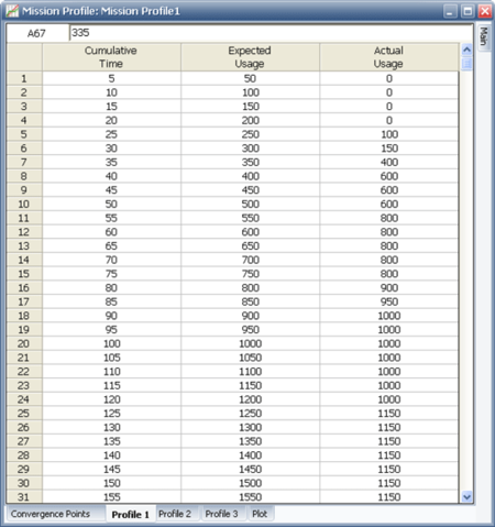
The next figure shows a portion of the expected and actual results for mission profile 1, as entered in the RGA software.
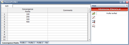
A graph exists for each of the three tasks in this example. Each graph has a line with the expected average as a function of hours, and the corresponding actual value. When the actual value for a task meets the expected value then it is a convergence for that task. A convergence point occurs when all of the tasks converge at the same time. At least three convergence points are required, one of which is the stopping point [math]\displaystyle{ T\,\! }[/math]. In our example, the total test time is 400 hours. The convergence points were chosen to be at 100, 250, 320 and 400 hours. The next figure shows the data sheet that contains the convergence points in the RGA software.
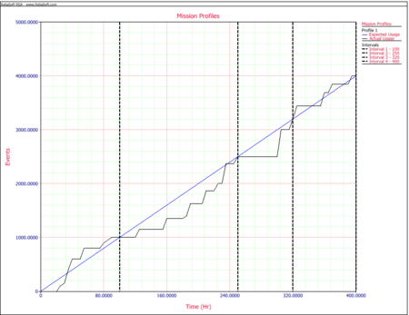
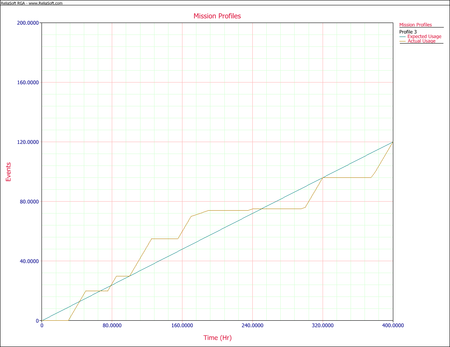
The testing profiles are managed so that at these times the actual operational test profile equals the expected values for the three tasks or falls within an acceptable range. The next graph shows the expected and actual gun firings.
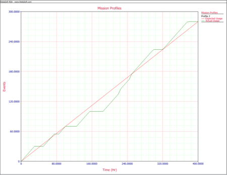
While the next two graphs show the expected and actual time in environments E1 and E2, respectively.
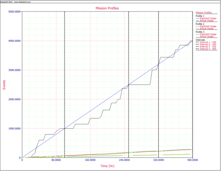
The objective of having the convergence points is to be able to apply the Crow extended model directly in such a way that the projection and other key reliability growth parameters can be estimated in a valid fashion. To do this, grouped data is applied using the Crow extended model. For reliability growth assessments using grouped data, only the information between time points in the testing is used. In our application, these time points are the convergence points 100, 250, 320, and 400. The next figure shows all three mission profiles plotted in the same graph, together with the convergence points.
The following table gives the grouped data input corresponding to the original data set.
| Grouped data at convergence points 100, 250, 320 and 400 hours | ||||||||
| Number at Event | Time to Event | Classification | Mode | Number at Event | Time to Event | Classification | Mode | |
|---|---|---|---|---|---|---|---|---|
| 3 | 100 | BC | 17 | 1 | 250 | BC | 26 | |
| 1 | 100 | BD | 1 | 1 | 250 | BD | 11 | |
| 1 | 100 | BC | 18 | 1 | 250 | BD | 12 | |
| 1 | 100 | BD | 2 | 3 | 320 | A | ||
| 1 | 100 | BD | 3 | 1 | 320 | BD | 1 | |
| 1 | 100 | BD | 4 | 1 | 320 | BD | 8 | |
| 1 | 100 | BC | 19 | 1 | 320 | BD | 6 | |
| 2 | 100 | BD | 5 | 1 | 320 | BC | 27 | |
| 1 | 100 | A | 1 | 320 | BD | 13 | ||
| 1 | 100 | BC | 20 | 1 | 320 | BD | 9 | |
| 1 | 100 | BD | 6 | 1 | 320 | BD | 4 | |
| 1 | 250 | BD | 7 | 3 | 400 | A | ||
| 3 | 250 | A | 1 | 400 | BD | 12 | ||
| 1 | 250 | BD | 8 | 2 | 400 | BD | 10 | |
| 1 | 250 | BC | 21 | 1 | 400 | BD | 5 | |
| 1 | 250 | BD | 2 | 1 | 400 | BD | 3 | |
| 1 | 250 | BC | 22 | 1 | 400 | BC | 28 | |
| 2 | 250 | BD | 9 | 1 | 400 | BD | 2 | |
| 2 | 250 | BD | 10 | 1 | 400 | BD | 8 | |
| 1 | 250 | BC | 23 | 1 | 400 | BD | 14 | |
| 1 | 250 | BC | 24 | 1 | 400 | BD | 15 | |
| 1 | 250 | BC | 25 | 1 | 400 | BD | 16 | |
The parameters of the Crow extended model for grouped data are then estimated, as explained in the Grouped Data section of the Crow Extended chapter. The following table shows the effectiveness factors (EFs) for the BD modes.
| Effectiveness Factors for delayed fixes | |
| Mode | Effectiveness Factor |
|---|---|
| 1 | 0.67 |
| 2 | 0.72 |
| 3 | 0.77 |
| 4 | 0.77 |
| 5 | 0.87 |
| 6 | 0.92 |
| 7 | 0.50 |
| 8 | 0.85 |
| 9 | 0.89 |
| 10 | 0.74 |
| 11 | 0.70 |
| 12 | 0.63 |
| 13 | 0.64 |
| 14 | 0.72 |
| 15 | 0.69 |
| 16 | 0.46 |
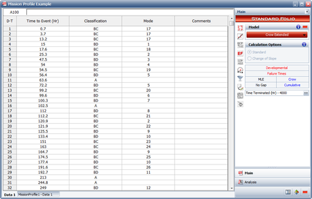
Using the failure times data sheet shown next, we can analyze this data set based on a specified mission profile. This will group the failure times data into groups based on the convergence points that have already been specified when constructing the mission profile.
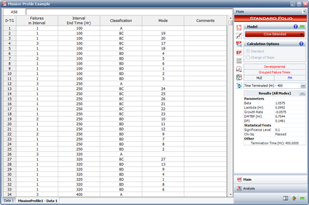
A new data sheet with the grouped data is created, as shown in the figure below and the calculated results based on the grouped data are as follows:
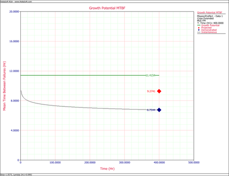
The following plot shows the instantaneous, demonstrated, projected and growth potential MTBF for the grouped data, based the mission profile grouping with intervals at the specified convergence points of the mission profile.

