Crow Extended

In reliability growth analysis, the Crow-AMSAA (NHPP) model assumes that the corrective actions for the observed failure modes are incorporated during the test (test-fix-test). However, in actual practice, fixes may be delayed until after the completion of the test (test-find-test) or some fixes may be implemented during the test while others are delayed (test-fix-find-test). At the end of a test phase, two reliability estimates are of concern: demonstrated reliability and projected reliability. The demonstrated reliability, which is based on data generated during the test phase, is an estimate of the system reliability for its configuration at the end of the test phase. The projected reliability measures the impact of the delayed fixes at the end of the current test phase.
Most of the reliability growth literature are concerned with procedures and models for calculating the demonstrated reliability, and very little attention has been paid to techniques for reliability projections. The procedure for making reliability projections utilizes engineering assessments of the effectiveness of the delayed fixes for each observed failure mode. These effectiveness factors are then used with the data generated during the test phase to obtain a projected estimate for the updated configuration by adjusting the number of failures observed during the test phase. The process of estimating the projected reliability is accomplished using the Crow Extended model. The Crow Extended model allows for a flexible growth strategy that can include corrective actions performed during the test, as well as delayed corrective actions. The test-find-test and test-fix-find-test scenarios are simply subsets of the Crow Extended model.
For developmental testing, the Crow Extended model can be applied when using any of the following data types:
- Failure Times Data
- Multiple Systems (Known Operating Times)
- Multiple Systems (Concurrent Operating Times)
- Multiple Systems with Dates
- Multiple Systems with Event Codes
- Grouped Failure Times
- Mixed Data
As the name implies, Crow Extended is simply an "extension" of the Crow-AMSAA (NHPP) model. The calculations for Crow Extended still incorporate the methods for Crow-AMSAA based on the data type, as described on the Crow-AMSAA (NHPP) page. The Crow-AMSAA model estimates the growth during the test, while the Crow Extended model accounts for the growth after the test based on the delayed corrective actions. Additional details regarding the calculations for the Crow Extended model are presented in the sections below.
Background
When a system is tested and failure modes are observed, management can make one of two possible decisions: to fix or to not fix the failure modes. Failure modes that are not fixed are called A modes and failure modes that receive a corrective action are called B modes. The A modes account for all failure modes that management considers to be not economical or not justified to receive corrective action. The B modes provide the assessment and management metric structure for corrective actions during and after a test. There are two types of B modes: BC modes, which are corrected during the test, and BD modes, which are corrected only at the end of the test. The management strategy is defined by how the corrective actions, if any, will be implemented. In summary, the classifications are defined as follows:
- A indicates that no corrective action was performed or will be performed (management chooses not to address for technical, financial or other reasons).
- BC indicates that the corrective action was implemented during the test. The analysis assumes that the effect of the corrective action was experienced during the test (as with other test-fix-test reliability growth analyses).
- BD indicates that the corrective action will be delayed until after the completion of the current test. BD modes will provide a jump in the system's MTBF at the termination time.
In terms of assessing a system's reliability, there are three specific metrics of interest:
- Demonstrated (or achieved) MTBF (DMTBF) is the system's instantaneous MTBF at the termination time.
- Projected MTBF (PMTBF) is the system's expected instantaneous MTBF after the implementation of the delayed corrective actions.
- Growth Potential MTBF (GPMTBF) is the maximum MTBF that can be attained for the system design and management strategy.
These metrics can also be displayed in RGA in terms of failure intensity (FI). The demonstrated MTBF is calculated using basically the same methods, depending on data type, as presented on the Crow-AMSAA (NHPP) page. Projected MTBF/FI and growth potential MTBF/FI are presented in detail in the sections below.
The following picture shows an example of data entered for the Crow Extended model.

As you can see, each failure is indicated with A, BC or BD in the Classification column. In addition, any number or text can be used to specify the failure mode. In this example, numbers were used in the Mode column for simplicity, but you could just as easily use "Seal Leak," or whatever designation you deem appropriate for identifying the mode. In RGA, a failure mode is defined as a problem and a cause.
Reliability growth is achieved by decreasing the failure intensity. The failure intensity for the A failure modes will not change; therefore, reliability growth can only be achieved by decreasing the BC and BD mode failure intensity. In general, the only part of the BD mode failure intensity that can be decreased is that which has been seen during testing, since the failure intensity due to BD modes that were unseen during testing still remains. The BC failure modes are corrected during test, and the BC failure intensity will not change any more at the end of test.
It is very important to note that once a BD failure mode is in the system, it is rarely totally eliminated by a corrective action. After a BD mode has been found and fixed, a certain percentage of the failure intensity will be removed, but a certain percentage of the failure intensity will generally remain. For each BD mode, an effectiveness factor (EF) is required to estimate how effective the corrective action will be in eliminating the failure intensity due to the failure mode. The EF is the fractional decrease in a mode's failure intensity after a corrective action has been made, and it must be a value between 0 and 1. It has been shown empirically that an average EF, [math]\displaystyle{ d\,\! }[/math], is about 70%. Therefore, about 30 percent, (i.e., 100 [math]\displaystyle{ (1-d)\,\! }[/math] percent), of the BD mode failure intensity will typically remain in the system after all of the corrective actions have been implemented. However, individual EFs for the failure modes may be larger or smaller than the average. The next figure displays the RGA software's Effectiveness Factor window where the effectiveness factors for each unique BD failure mode can be specified.

The EF does not account for the scenario where additional failure modes are created from the corrective actions. If this happens, then the actual EF will be lower than the assumed value. An EF greater than or equal to 0.9 indicates a significant improvement in a failure mode's MTBF (or reduction in failure intensity). This is indicative of a design change. The increase in a failure mode's MTBF, given an EF, can be calculated using:
- [math]\displaystyle{ Multiplier=\frac{1}{1-EF} }[/math]
Using this equation, an [math]\displaystyle{ EF=0.7\,\! }[/math] corresponds to an increase of 3.3X. Therefore, if a failure mode had an MTBF of 100 and a delayed fix was applied, an estimate of the failure mode's MTBF after the fix is equal to [math]\displaystyle{ \approx 333\,\! }[/math]. An [math]\displaystyle{ EF=0.9\,\! }[/math] corresponds to a 10X increase in the failure mode's MTBF. So there is a large increase between EF = 0.7 and EF = 0.9. Before assigning an EF to a BD mode, it is recommended to run a test to verify the fix and to validate the assumed EF value. Ideally, you want to have some sort of justification for using the entered EF value. If you do not know the EF value for each BD mode, then you can also specify a fixed EF which is then applied to all modes. The average value of EF = 0.7 is a good place to start, but if you want to be a bit more conservative, then an EF = 0.4, or a smaller value, could be used.
Test-Find-Test
Test-find-test is a testing strategy where all corrective actions are delayed until after the test. Therefore, there are not any BC modes when analyzing test-find-test data (only A and BD modes). This scenario is also called the Crow-AMSAA Projection model, but for the purposes of the RGA software, it is simply a special case of the Crow Extended model. The picture below presents the test-find-test scenario.

Since there are no fixes applied during the test, the assumption is that the system's MTBF does not change during the test. In other words, the system's MTBF is constant. The system should not be exhibiting an increasing or decreasing trend in its reliability if changes are not being made. Therefore, the assumption is that [math]\displaystyle{ \beta = 1\,\! }[/math]. RGA will return two [math]\displaystyle{ \beta\,\! }[/math] values; Beta (hyp) which always shows a value equal to 1 since this is the underlying assumption, and Beta which is the Crow-AMSAA (NHPP) estimate that considers all of the failure times. The assumption of [math]\displaystyle{ \beta = 1\,\! }[/math] can be verified by looking at the confidence bounds on [math]\displaystyle{ \beta\,\! }[/math]. If the confidence bounds on [math]\displaystyle{ \beta\,\! }[/math] include one, then you can fail to reject the hypothesis that [math]\displaystyle{ \beta = 1\,\! }[/math]. RGA does this check automatically and uses a confidence level equal to 1 minus the specified significance level to check if the confidence bounds on [math]\displaystyle{ \beta\,\! }[/math] include one. If the [math]\displaystyle{ \beta = 1\,\! }[/math] assumption is violated, then the value for Beta (hyp) will be displayed in red text. If the confidence bounds on [math]\displaystyle{ \beta\,\! }[/math] do not include 1, then the following questions should be considered as they relate to the data:
- If multiple systems were tested, did they have the same configuration throughout the test? Were the corrective actions applied to all systems?
- Were the test conditions consistent for each system?
- Was there a change in the failure definition?
- Any issues with data entry?
[math]\displaystyle{ \beta = 1\,\! }[/math] is then used to estimate the demonstrated MTBF of the system and it is also used in the goodness-of-fit tests.
Projected Failure Intensity
Suppose a system is subjected to development testing for a period of time, [math]\displaystyle{ T\,\! }[/math]. The system can be considered as consisting of two types of failure modes: A modes and BD modes. It is assumed that all BD modes are in series and fail independently according to the exponential distribution. Also assume that the rate of occurrence of A modes follows an exponential distribution with failure intensity [math]\displaystyle{ {{\lambda }_{A}}\,\! }[/math]. The system MTBF is constant throughout the test phase since all of the corrective actions are delayed until after the completion of the test. After the delayed fixes have been implemented, the system MTBF will then jump to a higher value.
Let [math]\displaystyle{ K\,\! }[/math] denote the total number of BD modes in the system, and let [math]\displaystyle{ {{\lambda }_{i}}\,\! }[/math] denote the failure intensity for the [math]\displaystyle{ {{i}^{th}}\,\! }[/math] BD mode, such that [math]\displaystyle{ i = 1,2,\ldots ,K\,\! }[/math]. Then, at time equal to zero, the system failure intensity [math]\displaystyle{ r(0)\,\! }[/math] is:
- [math]\displaystyle{ \begin{align} r(0)={{\lambda }_{A}}+{{\lambda }_{BD}} \end{align}\,\! }[/math]
where:
- [math]\displaystyle{ {{\lambda }_{BD}}=\underset{i=1}{\overset{K}{\mathop{\sum }}}\,{{\lambda }_{i}}\,\! }[/math].
During the test [math]\displaystyle{ (0,T)\,\! }[/math], a random number of [math]\displaystyle{ M\,\! }[/math] distinct BD modes will be observed, such that [math]\displaystyle{ M\le K\,\! }[/math]. Denote the effectiveness factor (EF) for the [math]\displaystyle{ {{i}^{th}}\,\! }[/math] BD mode as [math]\displaystyle{ {{d}_{i}}\,\! }[/math], [math]\displaystyle{ i = 1,2,\ldots ,K\,\! }[/math]. The effectiveness factor [math]\displaystyle{ {{d}_{i}}\,\! }[/math] is the percent decrease in [math]\displaystyle{ {{\lambda }_{i}}\,\! }[/math] after a corrective action has been made for the [math]\displaystyle{ {{i}^{th}}\,\! }[/math] BD mode. That is, the corrective action for the [math]\displaystyle{ {{i}^{th}}\,\! }[/math] BD mode removes [math]\displaystyle{ 100\times {{d}_{i}}\,\! }[/math] percent of the failure rate, and [math]\displaystyle{ 100\times (1-{{d}_{i}})\,\! }[/math] percent remains. The failure intensity for the [math]\displaystyle{ {{i}^{th}}\,\! }[/math] BD failure mode after a corrective action is [math]\displaystyle{ (1-{{d}_{i}}){{\lambda }_{i}}\,\! }[/math]. If corrective actions are taken on the [math]\displaystyle{ M\,\! }[/math] BD modes observed by time [math]\displaystyle{ T\,\! }[/math], then the system failure intensity is reduced from [math]\displaystyle{ r(0)\,\! }[/math] to:
- [math]\displaystyle{ \begin{align} r\left( T \right) = & {{\lambda }_{A}}+\underset{i=1}{\overset{M}{\mathop \sum }}\,\left( 1-{{d}_{i}} \right){{\lambda }_{i}}+({{\lambda }_{BD}}-\underset{i=1}{\overset{M}{\mathop \sum }}\,{{\lambda }_{i}}) \\ = & {{\lambda }_{A}}+{{\lambda }_{BD}}-\underset{i=1}{\overset{M}{\mathop \sum }}\,{{d}_{i}}{{\lambda }_{i}} \end{align}\,\! }[/math]
where:
- [math]\displaystyle{ \underset{i=1}{\overset{M}{\mathop{\sum }}}\,(1-{{d}_{i}}){{\lambda }_{i}}\,\! }[/math] is the failure intensity for the [math]\displaystyle{ M\,\! }[/math] modes after the corrective actions
- [math]\displaystyle{ ({{\lambda }_{BD}}-\underset{i=1}{\overset{M}{\mathop{\sum }}}\,{{\lambda }_{i}})\,\! }[/math] is the remaining failure intensity for all unseen BD modes
All [math]\displaystyle{ M\,\! }[/math] BD modes observed by test time [math]\displaystyle{ T\,\! }[/math] may not be fixed by time [math]\displaystyle{ T\,\! }[/math] so the actual failure intensity at time [math]\displaystyle{ T\,\! }[/math] may not be [math]\displaystyle{ r(T)\,\! }[/math]. However, [math]\displaystyle{ r(T)\,\! }[/math] can be viewed as the achieved failure intensity at time [math]\displaystyle{ T\,\! }[/math] if all fixes were updated and incorporated into the system. All of the fixes for the BD modes found during the test are incorporated as delayed fixes at the end of the test phase. Therefore, the system failure intensity is constant at [math]\displaystyle{ r(0)={{\lambda }_{A}}+{{\lambda }_{BD}}\,\! }[/math] through the test phase and will then jump to a lower value [math]\displaystyle{ r(T)\,\! }[/math] after the delayed fixes have been implemented. Let [math]\displaystyle{ {{N}_{A}}\,\! }[/math] and [math]\displaystyle{ {{N}_{BD}}\,\! }[/math] be the total number of A and BD failures observed during the test [math]\displaystyle{ (0,T)\,\! }[/math] and let [math]\displaystyle{ N={{N}_{A}}+{{N}_{BD}}\,\! }[/math]. In addition, there are [math]\displaystyle{ M\,\! }[/math] distinct BD modes observed during the test. After implementing the [math]\displaystyle{ M\,\! }[/math] fixes, the failure intensity for the system at time [math]\displaystyle{ T\,\! }[/math] (after the jump) is given by the function [math]\displaystyle{ r(T)\,\! }[/math].
[math]\displaystyle{ r(0)\,\! }[/math] is actually the demonstrated failure intensity, which is based on actual system performance of the hardware tested and not of some future configuration. A demonstrated reliability value should be determined at the end of each test phase. The demonstrated failure intensity is:
- [math]\displaystyle{ {{\hat{\lambda }}_{D}}(T)=r(0)=\frac{{{N}_{A}}+{{N}_{BD}}}{T}\,\! }[/math]
The demonstrated MTBF is given by:
- [math]\displaystyle{ \widehat{{MTBF}_{D}}={{[{{\hat{\lambda }}_{D}}(T)]}^{-1}}\,\! }[/math]
The detailed procedure for estimating [math]\displaystyle{ r(T)\,\! }[/math] is given in Crow [20] and is reviewed here.
Let [math]\displaystyle{ E[\cdot ]\,\! }[/math] denote the expected value:
- [math]\displaystyle{ E[r(T)]={{\lambda }_{A}}+\underset{i=1}{\overset{M}{\mathop \sum }}\,(1-{{d}_{i}}){{\lambda }_{i}}+\underset{i=1}{\overset{M}{\mathop \sum }}\,{{d}_{i}}{{\lambda }_{i}}{{e}^{-{{\lambda }_{i}}T}}\,\! }[/math]
Under realistic assumptions, [math]\displaystyle{ E[r(T)]\,\! }[/math] also may be expressed as:
- [math]\displaystyle{ E[r(T)]={{\lambda }_{A}}+\underset{i=1}{\overset{M}{\mathop \sum }}\,(1-{{d}_{i}}){{\lambda }_{i}}+\overline{d}h(T)\,\! }[/math]
where [math]\displaystyle{ \overline{d}\,\! }[/math] is the mean effectiveness factor and [math]\displaystyle{ h(T)\,\! }[/math] is the instantaneous rate at which a new BD mode will occur at time [math]\displaystyle{ T\,\! }[/math]. [math]\displaystyle{ \overline{d}h(T)\,\! }[/math] is the bias term (or sometimes called the 3rd term), such that:
- [math]\displaystyle{ B(T)=\overline{d}h(T)\,\! }[/math]
The mean [math]\displaystyle{ \overline{d}\,\! }[/math] is given by:
- [math]\displaystyle{ \overline{d}=\frac{1}{M}\underset{i=1}{\overset{M}{\mathop \sum }}\,{{d}_{i}}\,\! }[/math]
Therefore, the projected failure intensity [math]\displaystyle{ r(T)\,\! }[/math] is then estimated at the end of the test phase by:
- [math]\displaystyle{ \hat{r}(T)=\left( \frac{{{N}_{A}}}{T}+\underset{i=1}{\overset{M}{\mathop \sum }}\,(1-{{d}_{i}})\frac{{{N}_{i}}}{T} \right)+\overline{d}h(T)\,\! }[/math]
The projected MTBF is:
- [math]\displaystyle{ \widehat{{MTBF}_{P}}={{[r(T)]}^{-1}}\,\! }[/math]
Mathematical Formulation
As indicated previously, the failure intensity of the system at [math]\displaystyle{ t=0\,\! }[/math] is given by:
- [math]\displaystyle{ \begin{align} {{\lambda }_{System}}= & {{\lambda }_{A}}+{{\lambda }_{BD}} \\ = & {{\lambda }_{A}}+{{\lambda }_{B{{D}_{Seen}}}}+{{\lambda }_{B{{D}_{Unseen}}}} \end{align}\,\! }[/math]
The estimate for the projected failure intensity, after the corrective actions have been implemented, is then:
- [math]\displaystyle{ \begin{align} {{\lambda }_{\Pr ojected}}= & {{\lambda }_{A}}+\left( 1-d \right)\left( {{\lambda }_{BD}}-h\left( t \right) \right)+h\left( t \right)\\ = & {{\lambda }_{A}}+\left( 1-d \right){{\lambda }_{BD}}-\left( 1-d \right)h\left( t \right)+h\left( t \right)\\ = & {{\lambda }_{A}}+\left( 1-d \right){{\lambda }_{BD}}-h\left( t \right)+dh\left( t \right)+h\left( t \right)\\ = & {{\lambda }_{A}}+\left( 1-d \right){{\lambda }_{BD}}+dh\left( t \right) \end{align}\,\! }[/math]
This is the basic format of the equation for the projected failure intensity when the Crow Extended model is used with the test-find-test strategy.
h(t) Function
h(t) is defined as the unseen BD mode failure intensity. It is also defined as the rate at which new unique BD modes are being discovered. The maximum likelihood estimate of [math]\displaystyle{ h(t)\,\! }[/math] is calculated using:
- [math]\displaystyle{ \hat{h}\left( t \right)={{\hat{\lambda }}_{BD}}{{\overline{\beta }}_{BD}}{{t}^{{{{\overline{\beta }}}_{BD}}-1}}\,\! }[/math]
where [math]\displaystyle{ {\overline{\beta }_{BD}}\,\! }[/math] is the unbiased estimate. The unbiased estimate is always used when calculating [math]\displaystyle{ \hat{h}\left( t \right)\,\! }[/math].
The parameters of the [math]\displaystyle{ h(t)\,\! }[/math] function, [math]\displaystyle{ {{\beta }_{BD}}\,\! }[/math] and [math]\displaystyle{ {{\lambda }_{BD}}\,\! }[/math], are calculated using the first occurrence of each BD mode. In order to have growth, [math]\displaystyle{ {{\beta }_{BD}}\,\! }[/math] must be less than one. If [math]\displaystyle{ {{\beta }_{BD}}\,\! }[/math] is close to one then it is possible that the program could be in trouble since this indicates that there are very few repeat occurrences. In this case, each failure tends to be a unique mode. If [math]\displaystyle{ {{\beta }_{BD}}\,\! }[/math] is less than one then the rate at which new unique BD modes are occurring is decreasing.
Let [math]\displaystyle{ {{X}_{1}}\lt {{X}_{2}}\lt \ldots \lt {{X}_{M}}\lt T\,\! }[/math] denote the cumulative test times for the first occurrences of BD modes. Then, the maximum likelihood estimates of [math]\displaystyle{ {{\lambda }_{BD}}\,\! }[/math] and [math]\displaystyle{ {{\beta }_{BD}}\,\! }[/math] are:
- [math]\displaystyle{ {{\hat{\beta }}_{BD}}=\frac{M}{\underset{i=1}{\overset{M}{\mathop{\sum }}}\,\ln \left( \tfrac{T}{{{X}_{i}}} \right)}\,\! }[/math]
The unbiased estimate of [math]\displaystyle{ {{\beta }_{BD}}\,\! }[/math] is:
- [math]\displaystyle{ {{\bar{\beta }}_{BD}}=\frac{M-1}{M}{{\hat{\beta }}_{BD}}\,\! }[/math]
- [math]\displaystyle{ {{\hat{\lambda }}_{BD}}=\frac{M}{{{T}^{{{{\overline{\beta }}}_{BD}}}}}\,\! }[/math]
In particular, the maximum likelihood estimate for the rate of occurrence for the distinct BD modes at the termination time, [math]\displaystyle{ T\,\! }[/math], is:
- [math]\displaystyle{ \begin{align} \hat{h}(T) = & {{\hat{\lambda }}_{BD}}{{\overline{\beta }}_{BD}}{{T}^{{{\overline{\beta }}_{BD}}-1}} \\ = & \frac{M{{\overline{\beta }}_{BD}}}{T} \end{align}\,\! }[/math]
The parameters associated with [math]\displaystyle{ h(t)\,\! }[/math] can be viewed in RGA by selecting BD modes from the dropdown to the right of Results (All Modes) in the Results Area on the control panel to the right of the data sheet. The displayed value for the failure intensity, FI, is [math]\displaystyle{ h(T)\,\! }[/math].
Growth Potential
Growth Potential, when represented in terms of MTBF, is the maximum system reliability that can be attained for the system design with the current management strategy. The maximum MTBF will be attained when all [math]\displaystyle{ K\,\! }[/math] BD modes have been observed and fixed with EFs [math]\displaystyle{ {{d}_{i}}\,\! }[/math]. If the system is tested long enough then the failures that are observed in this case will be either repeat BD modes or A modes. In other words, there is not another unique BD mode to find within the system, and in most cases the growth potential is a value that may never actually be achieved. The growth potential can be thought of as an upper bound on the system's MTBF and ideally, should be about 30% above the system's requirement. As the system's MTBF gets closer to the growth potential, it becomes more difficult to increase the system's MTBF because it is taking more and more test time to propagate the next unique BD mode. The BD modes present opportunities for growth, but the rate of occurrence for unique BD modes goes down due to the decrease in [math]\displaystyle{ h(t)\,\! }[/math]. The growth potential is reached when [math]\displaystyle{ h(t)\,\! }[/math] is equal to zero. In other words, the difference between the projected failure intensity and the growth potential is [math]\displaystyle{ h(t)\,\! }[/math]. At about 2/3 of the growth potential it becomes increasingly difficult to increase the system's MTBF as [math]\displaystyle{ h(t)\,\! }[/math] function starts to flatten out.
The failure intensity [math]\displaystyle{ r(T)\,\! }[/math] will depend on the management strategy that determines the classification of the A and BD failure modes. The engineering effort applied to the corrective actions determines the effectiveness factors. In addition, [math]\displaystyle{ r(T)\,\! }[/math] depends on [math]\displaystyle{ h(t)\,\! }[/math], which is the rate at which problem failure modes are being seen during testing. [math]\displaystyle{ h(t)\,\! }[/math] drives the opportunity to take corrective actions based on the seen failure modes and it is an important factor in the overall reliability growth rate. The reliability growth potential is the limiting value of [math]\displaystyle{ r(T)\,\! }[/math] as [math]\displaystyle{ T\,\! }[/math] increases. This limit is the maximum MTBF that can be attained with the current management strategy. In terms of failure intensity, the growth potential is expressed by the following equation:
- [math]\displaystyle{ {{r}_{GP}}={{\lambda }_{A}}+\underset{i=1}{\overset{K}{\mathop \sum }}\,(1-{{d}_{i}}){{\lambda }_{i}}\,\! }[/math]
In terms of the MTBF, the growth potential is given by:
- [math]\displaystyle{ \begin{align} MTB{{F}_{GP}}=1/{{r}_{GP}} \end{align}\,\! }[/math]
The procedure for estimating the growth potential is as follows. Suppose that the system is tested for a period of time [math]\displaystyle{ T\,\! }[/math] and that [math]\displaystyle{ N\,\! }[/math] failures have been observed. According to the management strategy, [math]\displaystyle{ {{N}_{A}}\,\! }[/math] of these failures are A modes and [math]\displaystyle{ {{N}_{BD}}\,\! }[/math] of these failures are BD modes. For the BD modes, there will be [math]\displaystyle{ M\,\! }[/math] distinct fixes. As before, [math]\displaystyle{ {{N}_{i}}\,\! }[/math] is the total number of failures for the [math]\displaystyle{ {{i}^{th}}\,\! }[/math] BD mode and [math]\displaystyle{ {{d}_{i}}\,\! }[/math] is the corresponding assigned EF. From this data, the growth potential failure intensity is estimated by:
- [math]\displaystyle{ {{\hat{r}}_{GP}}(T)=\left( \frac{{{N}_{A}}}{T}+\underset{i=1}{\overset{M}{\mathop \sum }}\,(1-{{d}_{i}})\frac{{{N}_{i}}}{T} \right)\,\! }[/math]
The growth potential MTBF is estimated by:
- [math]\displaystyle{ M\hat{T}B{{F}_{GP}}={{[{{\hat{r}}_{GP}}]}^{-1}}\,\! }[/math]
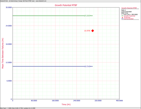
Example - Test-Find-Test Data
Consider the data in the first table below. A system was tested for [math]\displaystyle{ T=400\,\! }[/math] hours. There were a total of [math]\displaystyle{ N=42\,\! }[/math] failures and all corrective actions will be delayed until after the end of the 400 hour test. Each failure has been designated as either an A failure mode (the cause will not receive a corrective action) or a BD mode (the cause will receive a corrective action). There are [math]\displaystyle{ {{N}_{A}}=10\,\! }[/math] A mode failures and [math]\displaystyle{ {{N}_{BD}}=32\,\! }[/math] BD mode failures. In addition, there are [math]\displaystyle{ M=16\,\! }[/math] distinct BD failure modes, which means 16 distinct corrective actions will be incorporated into the system at the end of test. The total number of failures for the [math]\displaystyle{ {{j}^{th}}\,\! }[/math] observed distinct BD mode is denoted by [math]\displaystyle{ {{N}_{j}}\,\! }[/math], and the total number of BD failures during the test is [math]\displaystyle{ {{N}_{BD}}=\underset{j=1}{\overset{M}{\mathop{\sum }}}\,{{N}_{j}}\,\! }[/math]. These values and effectiveness factors are given in the second table
Do the following:
- Determine the projected MTBF and failure intensity.
- Determine the growth potential MTBF and failure intensity.
- Determine the demonstrated MTBF and failure intensity.
| Test-Find-Test Data | ||||||
| [math]\displaystyle{ i\,\! }[/math] | [math]\displaystyle{ {{X}_{i}}\,\! }[/math] | Mode | [math]\displaystyle{ i\,\! }[/math] | [math]\displaystyle{ {{X}_{i}}\,\! }[/math] | Mode | |
|---|---|---|---|---|---|---|
| 1 | 15 | BD1 | 22 | 260.1 | BD1 | |
| 2 | 25.3 | BD2 | 23 | 263.5 | BD8 | |
| 3 | 47.5 | BD3 | 24 | 273.1 | A | |
| 4 | 54 | BD4 | 25 | 274.7 | BD6 | |
| 5 | 56.4 | BD5 | 26 | 285 | BD13 | |
| 6 | 63.6 | A | 27 | 304 | BD9 | |
| 7 | 72.2 | BD5 | 28 | 315.4 | BD4 | |
| 8 | 99.6 | BD6 | 29 | 317.1 | A | |
| 9 | 100.3 | BD7 | 30 | 320.6 | A | |
| 10 | 102.5 | A | 31 | 324.5 | BD12 | |
| 11 | 112 | BD8 | 32 | 324.9 | BD10 | |
| 12 | 120.9 | BD2 | 33 | 342 | BD5 | |
| 13 | 125.5 | BD9 | 34 | 350.2 | BD3 | |
| 14 | 133.4 | BD10 | 35 | 364.6 | BD10 | |
| 15 | 164.7 | BD9 | 36 | 364.9 | A | |
| 16 | 177.4 | BD10 | 37 | 366.3 | BD2 | |
| 17 | 192.7 | BD11 | 38 | 373 | BD8 | |
| 18 | 213 | A | 39 | 379.4 | BD14 | |
| 19 | 244.8 | A | 40 | 389 | BD15 | |
| 20 | 249 | BD12 | 41 | 394.9 | A | |
| 21 | 250.8 | A | 42 | 395.2 | BD16 | |
| Effectiveness Factors for the Unique BD Modes | |||
| BD Mode | Number [math]\displaystyle{ {{N}_{j}}\,\! }[/math] | First Occurrence | EF [math]\displaystyle{ {{d}_{i}}\,\! }[/math] |
|---|---|---|---|
| 1 | 2 | 15.0 | .67 |
| 2 | 3 | 25.3 | .72 |
| 3 | 2 | 47.5 | .77 |
| 4 | 2 | 54.0 | .77 |
| 5 | 3 | 54.0 | .87 |
| 6 | 2 | 99.6 | .92 |
| 7 | 1 | 100.3 | .50 |
| 8 | 3 | 112.0 | .85 |
| 9 | 3 | 125.5 | .89 |
| 10 | 4 | 133.4 | .74 |
| 11 | 1 | 192.7 | .70 |
| 12 | 2 | 249.0 | .63 |
| 13 | 1 | 285.0 | .64 |
| 14 | 1 | 379.4 | .72 |
| 15 | 1 | 389.0 | .69 |
| 16 | 1 | 395.2 | .46 |
Solution
- The maximum likelihood estimates of [math]\displaystyle{ {{\beta }_{BD}}\,\! }[/math] and [math]\displaystyle{ {{\lambda }_{BD}}\,\! }[/math] are determined to be:
- [math]\displaystyle{ \begin{align} {{{\hat{\beta }}}_{BD}} = & \frac{M}{\underset{i=1}{\overset{M}{\mathop{\sum }}}\,\ln (\tfrac{T}{{{X}_{i}}})} \\ = & 0.7970 \\ {{{\hat{\lambda }}}_{BD}} = & 0.1350 \end{align}\,\! }[/math]
- [math]\displaystyle{ \begin{align} {{\overline{\beta }}_{BD}} = & \frac{M-1}{M}{{{\hat{\beta }}}_{BD}} \\ = & 0.7472 \end{align}\,\! }[/math]
- [math]\displaystyle{ \begin{align} r(T) = & \left( \frac{{{N}_{A}}}{T}+\underset{i=1}{\overset{M}{\mathop \sum }}\,(1-{{d}_{i}})\frac{{{N}_{i}}}{T} \right)+\overline{d}\left( \frac{M}{T}{{\overline{\beta }}_{BD}} \right) \\ = & 0.0661 \end{align}\,\! }[/math]
- [math]\displaystyle{ M\widehat{T}B{{F}_{P}}={{[r(T)]}^{-1}}=15.127\,\! }[/math]
- To estimate the maximum reliability that can be attained with this management strategy, use the following calculations.
- [math]\displaystyle{ \begin{align} {{N}_{A}}/T=0.0250 \end{align}\,\! }[/math]
- [math]\displaystyle{ \frac{1}{T}\underset{i=1}{\overset{16}{\mathop \sum }}\,(1-{{d}_{i}}){{N}_{i}}=0.0196\,\! }[/math]
- [math]\displaystyle{ \begin{align} {{\widehat{r}}_{GP}}(T) = & \left( \frac{{{N}_{A}}}{T}+\underset{i=1}{\overset{M}{\mathop \sum }}\,(1-{{d}_{i}})\frac{{{N}_{i}}}{T} \right) \\ = & 0.0250+0.0196 \\ = & 0.0446 \end{align}\,\! }[/math]
- [math]\displaystyle{ M\widehat{T}B{{F}_{GP}}={{[{{\widehat{r}}_{GP}}]}^{-1}}=22.4467\,\! }[/math]
- The demonstrated failure intensity and MTBF are estimated by:
- [math]\displaystyle{ \begin{align} {{\widehat{\lambda }}_{D}}(T) = & \frac{{{N}_{A}}+{{N}_{BD}}}{T} \\ = & \frac{42}{400} \\ = & 0.1050 \end{align}\,\! }[/math]
- [math]\displaystyle{ \begin{align} M\widehat{T}B{{F}_{D}} = & {{[{{\widehat{\lambda }}_{D}}(T)]}^{-1}} \\ = & 9.5238 \end{align}\,\! }[/math]


Test-Fix-Find-Test
Traditional reliability growth models provide assessments for two types of testing and corrective action strategies: test-fix-test and test-find-test. In test-fix-test, failure modes are found during testing and corrective actions for these modes are incorporated during the test. Data from this type of test can be modeled appropriately with the Crow-AMSAA model. In test-find-test, modes are found during testing, but all of the corrective actions are delayed and incorporated after the completion of the test. Data from this type of test can be modeled appropriately with the Crow-AMSAA Projection model, which was described above in the Test-Find-Test section. However, a common strategy involves a combination of these two approaches, where some corrective actions are incorporated during the test and some corrective actions are delayed and incorporated at the end of the test. This strategy is referred to as test-fix-find-test. Data from this test can be modeled appropriately with the Crow Extended reliability growth model, which is described next.
Recall that B failure modes are all failure modes that will receive a corrective action. In order to provide the assessment and management metric structure for corrective actions during and after a test, two types of B modes are defined. BC failure modes are corrected during the test and BD failure modes are delayed until the end of the test. Type A failure modes are defined as before; (i.e., those failure modes that will not receive a corrective action, either during or at the end of the test).
Development of the Crow Extended Model
Let [math]\displaystyle{ {{\lambda }_{BD}}\,\! }[/math] denote the constant failure intensity for the BD failure modes, and let [math]\displaystyle{ h(t|BD)\,\! }[/math] denote the first occurrence function for the BD failure modes. In addition, as before, let [math]\displaystyle{ K\,\! }[/math] be the number of BD failure modes, let [math]\displaystyle{ {{d}_{i}}\,\! }[/math] be the effectiveness factor for the [math]\displaystyle{ {{i}^{th}}\,\! }[/math] BD failure mode and let [math]\displaystyle{ \overline{d}\,\! }[/math] be the average effectiveness factor.
The Crow Extended model projected failure intensity is given by:
- [math]\displaystyle{ {{\lambda }_{EM}}={{\lambda }_{CA}}-{{\lambda }_{BD}}+\underset{i=1}{\overset{K}{\mathop \sum }}\,(1-{{d}_{i}}){{\lambda }_{i}}+\overline{d}h(T|BD)\,\! }[/math]
where [math]\displaystyle{ {{\lambda }_{CA}}=\lambda \beta {{T}^{\beta -1}}\,\! }[/math] is the achieved failure intensity at time [math]\displaystyle{ T\,\! }[/math].
The Crow Extended model projected MTBF is:
- [math]\displaystyle{ \begin{align} {{M}_{EM}}=1/{{\lambda }_{EM}} \end{align}\,\! }[/math]
This is the MTBF after the delayed fixes have been implemented. Under the extended reliability growth model, the demonstrated failure intensity before the delayed fixes is the first term, [math]\displaystyle{ {{\lambda }_{CA}}\,\! }[/math]. The demonstrated MTBF at time [math]\displaystyle{ T\,\! }[/math] before the delayed fixes is given by:
- [math]\displaystyle{ {{M}_{CA}}\text{ }={{[{{\lambda }_{CA}}]}^{-1}}\,\! }[/math]
If you assume that there are no delayed corrective actions (BD modes), then the model reduces to a special case of the Crow-AMSAA model where the achieved MTBF equals the projection, [math]\displaystyle{ \lambda_{CA}\,\! }[/math]. That is, there is no jump. If you assume that there are no corrective actions during the test (BC modes) then the model reduces to the test-find-test scenario described in the previous section.
Estimation of the Model
In the general estimation of the Crow Extended model, it is required that all failure times during the test are known. Furthermore, the ID of each A, BC and BD failure mode needs to be entered.
The estimate of the projected failure intensity for the Crow Extended model is given by:
- [math]\displaystyle{ {{\widehat{\lambda }}_{EM}}={{\widehat{\lambda }}_{CA}}-{{\widehat{\lambda }}_{BD}}+\underset{i=1}{\overset{M}{\mathop \sum }}\,(1-{{d}_{i}})\frac{{{N}_{i}}}{T}+\overline{d}\widehat{h}(T|BD)\,\! }[/math]
where [math]\displaystyle{ {{N}_{i}}\,\! }[/math] is the total number of failures for the [math]\displaystyle{ {{i}^{th}}\,\! }[/math] BD mode and [math]\displaystyle{ {{d}_{i}}\,\! }[/math] is the corresponding assigned EF. In order to obtain the first term, [math]\displaystyle{ {{\widehat{\lambda }}_{CA}}\,\! }[/math], fit all of the data (regardless of mode classification) to the Crow-AMSAA model to estimate [math]\displaystyle{ \widehat{\beta }\,\! }[/math] and [math]\displaystyle{ \widehat{\lambda }\,\! }[/math], thus:
- [math]\displaystyle{ {{\widehat{\lambda }}_{CA}}=\widehat{\lambda }\widehat{\beta }{{T}^{\widehat{\beta }-1}}\,\! }[/math]
The remaining terms are analyzed with the Crow Extended model, which is applied only to the BD data.
- [math]\displaystyle{ {{\widehat{\lambda }}_{BD}}=\frac{{{N}_{BD}}}{T}\,\! }[/math]
- [math]\displaystyle{ \begin{align} \widehat{h}(T|BD) = & {{\widehat{\lambda }}_{BD}}{{\widehat{\beta }}_{BD}}{{T}^{{{\widehat{\beta }}_{BD}}-1}} \\ = & \frac{M{{\widehat{\beta }}_{BD}}}{T} \end{align}\,\! }[/math]
[math]\displaystyle{ {{\widehat{\beta }}_{BD}}\,\! }[/math] is the unbiased estimated of [math]\displaystyle{ \beta \,\! }[/math] for the Crow-AMSAA model based on the first occurrence of [math]\displaystyle{ M\,\! }[/math] distinct BD modes.
The structure for the Crow Extended model includes the following special data analysis cases:
- Test-fix-test with no failure modes known or with BC failure modes known. With this type of data, the Crow Extended model will take the form of the traditional Crow-AMSAA analysis.
- Test-find-test with BD failure modes known. With this type of data, the Crow Extended model will take the form of the Crow-AMSAA Projection analysis described previously in the Test-Find-Test section.
- Test-fix-find-test with BC and BD failure modes known. With this type of data, the full capabilities of the Crow Extended model will be applied, as described in the following sections.
Reliability Growth Potential and Maturity Metrics
The growth potential and some maturity metrics for the Crow Extended model are calculated as follows.
- Initial system MTBF and failure intensity are given by:
- [math]\displaystyle{ {{\widehat{M}}_{I}}=\frac{\Gamma \left( 1+\tfrac{1}{\widehat{\beta }} \right)}{{{\widehat{\lambda }}^{\tfrac{1}{\widehat{\beta }}}}}\,\! }[/math]
and:
- [math]\displaystyle{ {{\widehat{\lambda }}_{I}}={{[{{\widehat{M}}_{I}}]}^{-1}}\,\! }[/math]
where [math]\displaystyle{ \widehat{\beta }\,\! }[/math] and [math]\displaystyle{ \widehat{\lambda }\,\! }[/math] are the estimators of the Crow-AMSAA model for all data regardless of the failure mode classification (i.e., A, BC or BD).
- The A mode failure intensity and MTBF are given by:
- [math]\displaystyle{ {{\widehat{\lambda }}_{A}}=\frac{{{N}_{A}}}{T}\,\! }[/math]
- [math]\displaystyle{ {{\widehat{M}}_{A}}={{[{{\widehat{\lambda }}_{A}}]}^{-1}}\,\! }[/math]
- The Initial BD mode failure intensity is given by:
- [math]\displaystyle{ {{\widehat{\lambda }}_{BD}}=\frac{{{N}_{BD}}}{T}\,\! }[/math]
- The BC mode initial failure intensity and MTBF are given by:
- [math]\displaystyle{ {{\widehat{\lambda }}_{I(BC)}}={{\widehat{\lambda }}_{I}}-{{\widehat{\lambda }}_{A}}-{{\widehat{\lambda }}_{BD}}\,\! }[/math]
- [math]\displaystyle{ {{\widehat{M}}_{I(BC)}}={{[{{\widehat{\lambda }}_{I(BC)}}]}^{-1}}\,\! }[/math]
- Failure intensity [math]\displaystyle{ h(T|BC)\,\! }[/math] and instantaneous MTBF [math]\displaystyle{ M(T|BC)\,\! }[/math] for new BC failure modes at the end of test time [math]\displaystyle{ T\,\! }[/math] are given by:
- [math]\displaystyle{ \widehat{h}(T|BC)=\widehat{\lambda }\widehat{\beta }{{T}^{\widehat{\beta }-1}}\,\! }[/math]
- [math]\displaystyle{ \widehat{M}(T|BC)={{[\widehat{h}(T|BC)]}^{-1}}\,\! }[/math]
where [math]\displaystyle{ \widehat{\beta }\,\! }[/math] and [math]\displaystyle{ \widehat{\lambda }\,\! }[/math] are the estimators of the Crow-AMSAA model for the first occurrence of distinct BC modes.
- Average effectiveness factor for BC failure modes is given by:
- [math]\displaystyle{ {{\widehat{d}}_{BC}}=\frac{\left[ \tfrac{N_{BC}^{\left( \tfrac{1}{{{{\hat{\beta }}}_{BC}}} \right)}}{\Gamma \left( 1+\tfrac{1}{{{{\hat{\beta }}}_{BC}}} \right)} \right]-{{N}_{BC}}}{\left[ \tfrac{N_{BC}^{\left( \tfrac{1}{{{{\hat{\beta }}}_{BC}}} \right)}}{\Gamma \left( 1+\tfrac{1}{{{{\hat{\beta }}}_{BC}}} \right)} \right]-{{M}_{BC}}}\,\! }[/math]
- where [math]\displaystyle{ {{N}_{BC}}\,\! }[/math] is the total number of observed BC modes, [math]\displaystyle{ {{M}_{BC}}\,\! }[/math] is the number of unique BC modes and [math]\displaystyle{ {{\hat{\beta }}_{BC}}\,\! }[/math] is the MLE for the first occurrence of distinct BC modes. If [math]\displaystyle{ {{\hat{\beta }}_{BC}}\ge 1\,\! }[/math] then [math]\displaystyle{ {{\widehat{d}}_{BC}}\,\! }[/math] equals zero.
- Growth potential failure intensity and growth potential MTBF are given by:
- [math]\displaystyle{ {{\widehat{\lambda }}_{GP}}={{\widehat{\lambda }}_{CA}}-{{\widehat{\lambda }}_{BD}}+\underset{i=1}{\overset{M}{\mathop \sum }}\,(1-{{d}_{i}})\frac{{{N}_{i}}}{T}\,\! }[/math]
- [math]\displaystyle{ {{\widehat{M}}_{GP}}={{[{{\widehat{\lambda }}_{GP}}]}^{-1}}\,\! }[/math]
Failure Mode Management Strategy
Management controls the resources for corrective actions. Consequently, the effectiveness factors are part of the management strategy. For the BD mode failure intensity that has been seen during development testing, 100 [math]\displaystyle{ d\,\! }[/math] percent will be removed and 100 [math]\displaystyle{ (1-d)\,\! }[/math] percent will remain in the system. Therefore, after the corrective actions have been made, the current system instantaneous failure intensity consists of the failure intensity due to the A modes plus the failure intensity for the unseen BC modes, and plus the failure intensity for the unseen BD modes plus the failure intensity for the BD modes that have been seen. The following pie chart shows how the system's instantaneous failure intensity can be broken down into its individual pieces based on the current failure mode strategy.

Keep in mind that the individual components of the system's instantaneous failure intensity will depend on the classifications defined in the data. For example, if BC modes are not present within the data, then the BC mode MTBF will not be a part of the overall system MTBF. The individual pieces of the pie, as shown in the above figure, are calculated using the following equations.
Let:
- [math]\displaystyle{ \hat{r}(T)=\hat{\lambda }\hat{\beta }{{T}^{\hat{\beta }-1}}\,\! }[/math]
where [math]\displaystyle{ T\,\! }[/math] is the test time and [math]\displaystyle{ \hat{\beta }\,\! }[/math] and [math]\displaystyle{ \hat{\lambda }\,\! }[/math] are the maximum likelihood estimates of the Crow-AMSAA model for all of the data. [math]\displaystyle{ \hat{\beta }\,\! }[/math] is the biased estimate of [math]\displaystyle{ \beta \,\! }[/math]. Therefore:
- [math]\displaystyle{ \hat{\beta }=\frac{N}{\underset{i=1}{\overset{N}{\mathop{\sum }}}\,\ln \left( \tfrac{T}{{{X}_{i}}} \right)}\,\! }[/math]
- [math]\displaystyle{ \hat{\lambda }=\frac{N}{{{T}^{{\hat{\beta }}}}}\,\! }[/math]
where [math]\displaystyle{ N\,\! }[/math] is the total number of failures, and [math]\displaystyle{ {{X}_{i}}\,\! }[/math] is the [math]\displaystyle{ {{i}^{th}}\,\! }[/math] time-to-failure. Let the successive failures [math]\displaystyle{ 0\lt {{X}_{1}}\lt {{X}_{2}}\lt \ldots \lt {{X}_{3}}\lt {{X}_{N}}\,\! }[/math] be partitioned into the A mode failures ( [math]\displaystyle{ {{N}_{A}}\,\! }[/math] ), BC first occurrence failures ( [math]\displaystyle{ {{N}_{BCF}}\,\! }[/math] ), BC remaining failures ( [math]\displaystyle{ {{N}_{BCR}}\,\! }[/math] ), BD first occurrence failure ( [math]\displaystyle{ {{N}_{BDF}}\,\! }[/math] ) and the BD remaining failures ( [math]\displaystyle{ {{N}_{BDR}}\,\! }[/math] ). For continuous data, each portion of the pie chart, due to each of the modes, is calculated as follows:
- A modes
- [math]\displaystyle{ A=\left( \frac{T}{{{N}^{2}}} \right)\left[ \underset{i=1}{\overset{{{N}_{A}}}{\mathop \sum }}\,\ln \left( \frac{T}{{{X}_{Ai}}} \right) \right]\hat{r}(T)\,\! }[/math]
- BC modes unseen
- [math]\displaystyle{ B{{C}_{unseen}}=\left( \frac{T}{{{N}^{2}}} \right)\left[ \underset{i=1}{\overset{{{N}_{BCF}}}{\mathop \sum }}\,\ln \left( \frac{T}{{{X}_{BCFi}}} \right) \right]\hat{r}(T)\,\! }[/math]
- BC modes seen
- [math]\displaystyle{ B{{C}_{seen}}=\left( \frac{T}{{{N}^{2}}} \right)\left[ \underset{i=1}{\overset{{{N}_{BCR}}}{\mathop \sum }}\,\ln \left( \frac{T}{{{X}_{BCRi}}} \right) \right]\hat{r}(T)\,\! }[/math]
- BD modes unseen
- [math]\displaystyle{ B{{D}_{unseen}}=\left( \frac{T}{{{N}^{2}}} \right)\left[ \underset{i=1}{\overset{{{N}_{BDF}}}{\mathop \sum }}\,\ln \left( \frac{T}{{{X}_{BDFi}}} \right) \right]\hat{r}(T)\,\! }[/math]
- BD modes seen
- [math]\displaystyle{ B{{D}_{seen}}=\left( \frac{T}{{{N}^{2}}} \right)\left[ \underset{i=1}{\overset{{{N}_{BDR}}}{\mathop \sum }}\,\ln \left( \frac{T}{{{X}_{BDRi}}} \right) \right]\hat{r}(T)\,\! }[/math]
- BD modes remain
- [math]\displaystyle{ \begin{align} B{{D}_{remain}} = & \left( 1-\frac{1}{M}\underset{i=1}{\overset{M}{\mathop \sum }}\,{{d}_{i}} \right)\cdot B{{D}_{seen}} \\ = & \left( 1-\overline{d} \right)\cdot B{{D}_{seen}} \end{align}\,\! }[/math]
- BD modes removed
- [math]\displaystyle{ \begin{align} B{{D}_{removed}} = & \frac{1}{M}\underset{i=1}{\overset{M}{\mathop \sum }}\,{{d}_{i}}\cdot B{{D}_{seen}} \\ = & \overline{d}\cdot B{{D}_{seen}} \end{align}\,\! }[/math]
For grouped data, the maximum likelihood estimates of [math]\displaystyle{ \beta \,\! }[/math] and [math]\displaystyle{ \lambda \,\! }[/math] from the Crow-AMSAA (NHPP) model are calculated such that the following equations are satisfied:
- [math]\displaystyle{ \underset{i=1}{\overset{K}{\mathop \sum }}\,{{N}_{i}}\left[ \frac{t_{i}^{{\hat{\beta }}}\ln ({{t}_{i}})-t_{i-1}^{{\hat{\beta }}}\ln ({{t}_{i-1}})}{t_{i}^{{\hat{\beta }}}-t_{i-1}^{{\hat{\beta }}}}-\ln T \right]=0\,\! }[/math]
- [math]\displaystyle{ \hat{\lambda }=\frac{N}{T_{K}^{{\hat{\beta }}}}\,\! }[/math]
where [math]\displaystyle{ K\,\! }[/math] is the number of groups and [math]\displaystyle{ N=\underset{i=1}{\overset{K}{\mathop{\sum }}}\,{{N}_{i}}\,\! }[/math].
- A modes
- [math]\displaystyle{ A=\left( \frac{T}{{{N}^{2}}} \right)\left[ {{N}_{A}}\ln (T)-\underset{i=1}{\overset{K}{\mathop \sum }}\,\frac{{{N}_{Ai}}}{{\hat{\beta }}}\left( \frac{t_{i}^{{\hat{\beta }}}\ln (t_{i}^{{\hat{\beta }}})-t_{i-1}^{{\hat{\beta }}}\ln (t_{i-1}^{{\hat{\beta }}})}{t_{i}^{{\hat{\beta }}}-t_{i-1}^{{\hat{\beta }}}}-1 \right) \right]\hat{r}(T)\,\! }[/math]
- BC modes unseen
- [math]\displaystyle{ B{{C}_{unseen}}=\left( \frac{T}{{{N}^{2}}} \right)\left[ {{N}_{BCF}}\ln (T)-\underset{i=1}{\overset{K}{\mathop \sum }}\,\frac{{{N}_{BCFi}}}{{\hat{\beta }}}\left( \frac{t_{i}^{{\hat{\beta }}}\ln (t_{i}^{{\hat{\beta }}})-t_{i-1}^{{\hat{\beta }}}\ln (t_{i-1}^{{\hat{\beta }}})}{t_{i}^{{\hat{\beta }}}-t_{i-1}^{{\hat{\beta }}}}-1 \right) \right]\hat{r}(T)\,\! }[/math]
- BC modes seen
- [math]\displaystyle{ B{{C}_{seen}}=\left( \frac{T}{{{N}^{2}}} \right)\left[ {{N}_{BCR}}\ln (T)-\underset{i=1}{\overset{K}{\mathop \sum }}\,\frac{{{N}_{BCRi}}}{{\hat{\beta }}}\left( \frac{t_{i}^{{\hat{\beta }}}\ln (t_{i}^{{\hat{\beta }}})-t_{i-1}^{{\hat{\beta }}}\ln (t_{i-1}^{{\hat{\beta }}})}{t_{i}^{{\hat{\beta }}}-t_{i-1}^{{\hat{\beta }}}}-1 \right) \right]\hat{r}(T)\,\! }[/math]
- BD modes unseen
- [math]\displaystyle{ B{{D}_{unseen}}=\left( \frac{T}{{{N}^{2}}} \right)\left[ {{N}_{BDF}}\ln (T)-\underset{i=1}{\overset{K}{\mathop \sum }}\,\frac{{{N}_{BDFi}}}{{\hat{\beta }}}\left( \frac{t_{i}^{{\hat{\beta }}}\ln (t_{i}^{{\hat{\beta }}})-t_{i-1}^{{\hat{\beta }}}\ln (t_{i-1}^{{\hat{\beta }}})}{t_{i}^{{\hat{\beta }}}-t_{i-1}^{{\hat{\beta }}}}-1 \right) \right]\hat{r}(T)\,\! }[/math]
- BD modes seen
- [math]\displaystyle{ B{{D}_{seen}}=\left( \frac{T}{{{N}^{2}}} \right)\left[ {{N}_{BDR}}\ln (T)-\underset{i=1}{\overset{K}{\mathop \sum }}\,\frac{{{N}_{BDRi}}}{{\hat{\beta }}}\left( \frac{t_{i}^{{\hat{\beta }}}\ln (t_{i}^{{\hat{\beta }}})-t_{i-1}^{{\hat{\beta }}}\ln (t_{i-1}^{{\hat{\beta }}})}{t_{i}^{{\hat{\beta }}}-t_{i-1}^{{\hat{\beta }}}}-1 \right) \right]\hat{r}(T)\,\! }[/math]
- BD modes remain
- [math]\displaystyle{ \begin{align} B{{D}_{remain}} = & \left( 1-\frac{1}{M}\underset{i=1}{\overset{M}{\mathop \sum }}\,{{d}_{i}} \right)\cdot B{{D}_{seen}} \\ = & \left( 1-\overline{d} \right)\cdot B{{D}_{seen}} \end{align}\,\! }[/math]
- BD modes removed
- [math]\displaystyle{ \begin{align} B{{D}_{removed}} = & \frac{1}{M}\underset{i=1}{\overset{M}{\mathop \sum }}\,{{d}_{i}}\cdot B{{D}_{seen}} \\ = & \overline{d}\cdot B{{D}_{seen}} \end{align}\,\! }[/math]
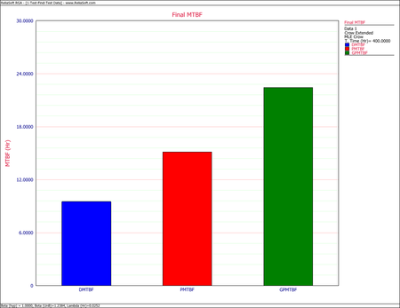
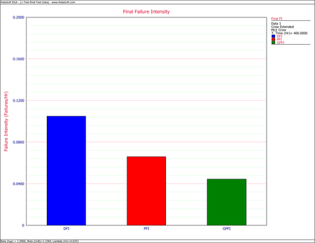
Example - Test-Fix-Find-Test Data
Consider the data given in the first table below. There were 56 total failures and [math]\displaystyle{ T=400\,\! }[/math]. The effectiveness factors of the unique BD modes are given in the second table. Determine the following:
- Calculate the demonstrated MTBF and failure intensity.
- Calculate the projected MTBF and failure intensity.
- What is the rate at which unique BD modes are being generated during this test?
- If the test continues for an additional 50 hours, what is the minimum number of new unique BD modes expected to be generated?
| Test-Fix-Find-Test Data | |||||
| [math]\displaystyle{ i\,\! }[/math] | [math]\displaystyle{ {{X}_{i}}\,\! }[/math] | Mode | [math]\displaystyle{ i\,\! }[/math] | [math]\displaystyle{ {{X}_{i}}\,\! }[/math] | Mode |
|---|---|---|---|---|---|
| 1 | 0.7 | BC17 | 29 | 192.7 | BD11 |
| 2 | 3.7 | BC17 | 30 | 213 | A |
| 3 | 13.2 | BC17 | 31 | 244.8 | A |
| 4 | 15 | BD1 | 32 | 249 | BD12 |
| 5 | 17.6 | BC18 | 33 | 250.8 | A |
| 6 | 25.3 | BD2 | 34 | 260.1 | BD1 |
| 7 | 47.5 | BD3 | 35 | 263.5 | BD8 |
| 8 | 54 | BD4 | 36 | 273.1 | A |
| 9 | 54.5 | BC19 | 37 | 274.7 | BD6 |
| 10 | 56.4 | BD5 | 38 | 282.8 | BC27 |
| 11 | 63.6 | A | 39 | 285 | BD13 |
| 12 | 72.2 | BD5 | 40 | 304 | BD9 |
| 13 | 99.2 | BC20 | 41 | 315.4 | BD4 |
| 14 | 99.6 | BD6 | 42 | 317.1 | A |
| 15 | 100.3 | BD7 | 43 | 320.6 | A |
| 16 | 102.5 | A | 44 | 324.5 | BD12 |
| 17 | 112 | BD8 | 45 | 324.9 | BD10 |
| 18 | 112.2 | BC21 | 46 | 342 | BD5 |
| 19 | 120.9 | BD2 | 47 | 350.2 | BD3 |
| 20 | 121.9 | BC22 | 48 | 355.2 | BC28 |
| 21 | 125.5 | BD9 | 49 | 364.6 | BD10 |
| 22 | 133.4 | BD10 | 50 | 364.9 | A |
| 23 | 151 | BC23 | 51 | 366.3 | BD2 |
| 24 | 163 | BC24 | 52 | 373 | BD8 |
| 25 | 164.7 | BD9 | 53 | 379.4 | BD14 |
| 26 | 174.5 | BC25 | 54 | 389 | BD15 |
| 27 | 177.4 | BD10 | 55 | 394.9 | A |
| 28 | 191.6 | BC26 | 56 | 395.2 | BD16 |
| Effectiveness Factors for the Unique BD Modes | |
| BD Mode | EF [math]\displaystyle{ {{d}_{i}}\,\! }[/math] |
|---|---|
| 1 | .67 |
| 2 | .72 |
| 3 | .77 |
| 4 | .77 |
| 5 | .87 |
| 6 | .92 |
| 7 | .50 |
| 8 | .85 |
| 9 | .89 |
| 10 | .74 |
| 11 | .70 |
| 12 | .63 |
| 13 | .64 |
| 14 | .72 |
| 15 | .69 |
| 16 | .46 |
Solution
- In order to obtain [math]\displaystyle{ {{\widehat{\lambda }}_{CA}}\,\! }[/math], use the traditional Crow-AMSAA model for test-fix-test to fit all 56 data points, regardless of the failure mode classification to get:
- [math]\displaystyle{ \begin{align} \widehat{\beta }= & 0.91026 \\ \widehat{\lambda }= & 0.23969 \end{align}\,\! }[/math]
- [math]\displaystyle{ \begin{align} {{\widehat{\lambda }}_{CA}} = & \widehat{\lambda }\widehat{\beta }{{T}^{\widehat{\beta }-1}} \\ = & 0.23969\times 0.91026\times {{400}^{(0.91026-1)}} \\ = & 0.12744 \end{align}\,\! }[/math]
- [math]\displaystyle{ {{\widehat{M}}_{CA}}={{[{{\widehat{\lambda }}_{CA}}]}^{-1}}=7.84708\,\! }[/math]
- For this data set, [math]\displaystyle{ M=16\,\! }[/math] and [math]\displaystyle{ T=400\,\! }[/math].
- [math]\displaystyle{ {{\widehat{\lambda }}_{BD}}=\frac{{{N}_{BD}}}{T}=\frac{32}{400}=0.08\,\! }[/math]
- [math]\displaystyle{ \overline{d}=\underset{i=1}{\overset{M}{\mathop \sum }}\,{{d}_{i}}/M=0.72125\,\! }[/math]
- [math]\displaystyle{ \underset{i=1}{\overset{16}{\mathop \sum }}\,(1-{{d}_{i}}){{N}_{i}}/T=0.01955\,\! }[/math]
- [math]\displaystyle{ \begin{align} {{{\hat{\beta }}}_{BD}}= & 0.74715 \\ {{{\hat{\lambda }}}_{BD}} = & 0.18197 \end{align}\,\! }[/math]
- [math]\displaystyle{ \overline{d}\widehat{h}(T|BD)=0.0215\,\! }[/math]
- [math]\displaystyle{ \begin{align} {{\widehat{\lambda }}_{EM}} = & {{\widehat{\lambda }}_{CA}}-{{\widehat{\lambda }}_{BD}}+\underset{i=1}{\overset{K}{\mathop \sum }}\,(1-{{d}_{i}})\frac{{{N}_{i}}}{T}+\overline{d}\widehat{h}(T|BD) \\ = & 0.12744-0.08+0.0196+0.0215 \\ = & 0.08854 \end{align}\,\! }[/math]
- [math]\displaystyle{ \begin{align} {{\widehat{M}}_{EM}} = & {{[{{\widehat{\lambda }}_{EM}}]}^{-1}} \\ = & 11.29418 \end{align}\,\! }[/math]
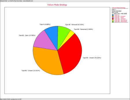
This pie chart shows that 9.48% of the system's failure intensity has been left in (A modes), 31.81% of the failure intensity due to the BC modes has not been seen yet and 13.40% was removed during the test (BC modes - seen). In addition, 33.23% of the failure intensity due to the BD modes has not been seen yet, 3.37% will remain in the system since the corrective actions will not be completely effective at eliminating the identified failure modes, and 8.72% will be removed after the delayed corrective actions.
- The rate at which unique BD modes are being generated is equal to [math]\displaystyle{ h{{(T|BD)}^{-1}}\,\! }[/math], where:
- [math]\displaystyle{ \begin{align} h{{(T|BD)}^{-1}} = & \frac{1}{{{\widehat{\lambda }}_{BD}}{{\widehat{\beta }}_{BD}}{{T}^{{{\widehat{\beta }}_{BD}}-1}}} \\ = & \frac{T}{M{{\widehat{\beta }}_{BD}}} \\ = & 33.4605 \end{align}\,\! }[/math]
- Unique BD modes are being generated every 33.4605 hours. If the test continues for another 50 hours, then at least one new unique BD mode would be expected to be seen from this additional testing.
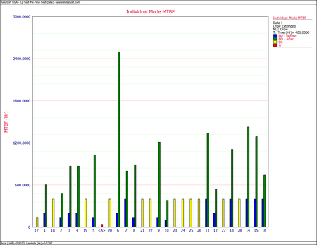
As shown in the next figure, the MTBF of each individual failure mode can be plotted, and the failure modes with the lowest MTBF can be identified. These are the failure modes that cause the majority of the system failures.


Confidence Bounds
The RGA software provides two methods to estimate the confidence bounds for the Crow Extended model when applied to developmental testing data. The Fisher Matrix approach is based on the Fisher Information Matrix and is commonly employed in the reliability field. The Crow bounds were developed by Dr. Larry Crow.
See the Crow Extended Confidence Bounds chapter for details on how these confidence bounds are calculated.
Confidence Bounds Example
Calculate the 2-sided 90% confidence bounds on the demonstrated, projected and growth potential failure intensity for the Test-Find-Test data given above.
Solution
The estimated demonstrated failure intensity is [math]\displaystyle{ {{\widehat{\lambda }}_{D}}(T)=\tfrac{{{N}_{A}}+{{N}_{B}}}{T}=0.1050\,\! }[/math]. Based on this value, the Fisher Matrix confidence bounds for the demonstrated failure intensity at the 90% confidence level are:
- [math]\displaystyle{ \begin{align} {{[{{\lambda }_{D}}(T)]}_{L}} = & {{{\hat{\lambda }}}_{D}}(T)+\frac{{{C}^{2}}}{2}-\sqrt{{{{\hat{\lambda }}}_{D}}(T){{C}^{2}}+\frac{{{C}^{4}}}{4}} \\ = & 0.08152 \end{align}\,\! }[/math]
- [math]\displaystyle{ \begin{align} {{[{{\lambda }_{D}}(T)]}_{U}} = & {{{\hat{\lambda }}}_{D}}(T)+\frac{{{C}^{2}}}{2}+\sqrt{{{{\hat{\lambda }}}_{D}}(T){{C}^{2}}+\frac{{{C}^{4}}}{4}} \\ = & 0.13525 \end{align}\,\! }[/math]
The Crow confidence bounds for the demonstrated failure intensity at the 90% confidence level are:
- [math]\displaystyle{ \begin{align} {{[{{\lambda }_{D}}(T)]}_{L}} = & {{\widehat{\lambda }}_{D}}(T)\frac{\chi _{(2N,1-\alpha /2)}^{2}}{2N} \\ = & 0.07985 \\ {{[{{\lambda }_{D}}(T)]}_{U}} = & {{\widehat{\lambda }}_{D}}(T)\frac{\chi _{(2N,\alpha /2)}^{2}}{2N} \\ = & 0.13299 \end{align}\,\! }[/math]
The projected failure intensity is:
- [math]\displaystyle{ \begin{align} \hat{\lambda_{p}} &= \frac{N_{i}}{T}+\sum_{i=1}^{M}(1-d_{i})\frac{N}{T}+\overline{d}\left(\frac{M}{T}\overline{\beta} \right )\\ &= 0.06611 \end{align} }[/math]
Based on this value, the Fisher Matrix confidence bounds at the 90% confidence level for the projected failure intensity are:
- [math]\displaystyle{ \begin{align} {{[{{{\hat{\lambda }}}_{P}}(T)]}_{L}} = & {{{\hat{\lambda }}}_{P}}(T){{e}^{{{z}_{\alpha }}\sqrt{Var({{{\hat{\lambda }}}_{P}}(T))}/{{{\hat{\lambda }}}_{P}}(T)}} \\ = & 0.04902 \end{align}\,\! }[/math]
- [math]\displaystyle{ \begin{align} {{[{{{\hat{\lambda }}}_{P}}(T)]}_{U}} = & {{{\hat{\lambda }}}_{P}}(T){{e}^{-{{z}_{\alpha }}\sqrt{Var({{{\hat{\lambda }}}_{P}}(T))}/{{{\hat{\lambda }}}_{P}}(T)}} \\ = & 0.08915 \end{align}\,\! }[/math]
The Crow confidence bounds for the projected failure intensity are:
- [math]\displaystyle{ \begin{align} {{[{{\lambda }_{P}}(T)]}_{L}} = & {{{\hat{\lambda }}}_{P}}(T)+\frac{{{C}^{2}}}{2}-\sqrt{{{{\hat{\lambda }}}_{P}}(T)\cdot {{C}^{2}}+\frac{{{C}^{4}}}{4}} \\ = & 0.04807 \\ {{[{{\lambda }_{P}}(T)]}_{U}} = & {{{\hat{\lambda }}}_{P}}(T)+\frac{{{C}^{2}}}{2}+\sqrt{{{{\hat{\lambda }}}_{P}}(T)\cdot \ \,{{C}^{2}}+\frac{{{C}^{4}}}{4}} \\ = & 0.09090 \end{align}\,\! }[/math]
The growth potential failure intensity is:
- [math]\displaystyle{ \widehat{r}_{GP} (T) = \left (\frac{N_A}{T} + \sum_{i=1}^M (1-d_i) \tfrac{N_i}{T} \right ) = 0.04455 \,\! }[/math].
Based on this value, the Fisher Matrix and Crow confidence bounds at the 90% confidence level for the growth potential failure intensity are:
- [math]\displaystyle{ \begin{align} {{r}_{L}} = & {{{\hat{r}}}_{GP}}+\frac{{{C}^{2}}}{2}-\sqrt{{{{\hat{r}}}_{GP}}{{C}^{2}}+\frac{{{C}^{4}}}{4}} \\ = & 0.03020 \\ {{r}_{U}} = & {{{\hat{r}}}_{GP}}+\frac{{{C}^{2}}}{2}+\sqrt{{{{\hat{r}}}_{GP}}{{C}^{2}}+\frac{{{C}^{4}}}{4}} \\ = & 0.0656 \end{align}\,\! }[/math]
The figure below shows the Fisher Matrix confidence bounds at the 90% confidence level for the demonstrated, projected and growth potential failure intensity.

The following figure shows these bounds based on the Crow method.

Another Confidence Bounds Example
Calculate the 2-sided confidence bounds at the 90% confidence level on the demonstrated, projected and growth potential MTBF for the Test-Fix-Find-Test data given above.
Solution
For this example, there are A, BC and BD failure modes, so the estimated demonstrated failure intensity, [math]\displaystyle{ {{\hat{\lambda }}_{D}}(T)\,\! }[/math], is simply the Crow-AMSAA model applied to all A, BC, and BD data.
- [math]\displaystyle{ {{\hat{\lambda }}_{D}}(T)={{\widehat{\lambda }}_{CA}}=\widehat{\lambda }\widehat{\beta }{{T}^{\widehat{\beta }-1}}=0.12744\,\! }[/math]
Therefore, the demonstrated MTBF is:
- [math]\displaystyle{ MTB{{F}_{D}}={{[{{\hat{\lambda }}_{D}}(T)]}^{-1}}=7.84708\,\! }[/math]
Based on this value, the Fisher Matrix confidence bounds for the demonstrated failure intensity at the 90% confidence level are:
- [math]\displaystyle{ \begin{align} {{[{{\lambda }_{D}}(T)]}_{L}} = & {{{\hat{\lambda }}}_{CA}}(T){{e}^{{{z}_{\alpha }}\sqrt{Var({{{\hat{\lambda }}}_{CA}}(T))}/{{{\hat{\lambda }}}_{CA}}(T)}} \\ = & 0.09339 \end{align}\,\! }[/math]
- [math]\displaystyle{ \begin{align} {{[{{\lambda }_{D}}(T)]}_{U}} = & {{{\hat{\lambda }}}_{CA}}(T){{e}^{-{{z}_{\alpha }}\sqrt{Var({{{\hat{\lambda }}}_{CA}}(T))}/{{{\hat{\lambda }}}_{CA}}(T)}} \\ = & 0.17390 \end{align}\,\! }[/math]
The Fisher Matrix confidence bounds for the demonstrated MTBF at the 90% confidence level are:
- [math]\displaystyle{ \begin{align} MTB{{F}_{{{D}_{L}}}} = & \frac{1}{{{[{{\lambda }_{D}}(T)]}_{U}}} \\ = & 5.75054 \\ MTB{{F}_{{{D}_{U}}}} = & \frac{1}{{{[{{\lambda }_{D}}(T)]}_{L}}} \\ = & 10.70799 \end{align}\,\! }[/math]
The Crow confidence bounds for the demonstrated MTBF at the 90% confidence level are:
- [math]\displaystyle{ \begin{align} MTB{{F}_{{{D}_{L}}}} = & \frac{1}{{{[{{\lambda }_{D}}(T)]}_{U}}} \\ = & \frac{1}{{{\widehat{\lambda }}_{D}}(T)\tfrac{{{\chi }^{2}}(2N,\alpha /2)}{2N}} \\ = & 5.6325 \\ MTB{{F}_{{{D}_{U}}}} = & \frac{1}{{{[{{\lambda }_{D}}(T)]}_{L}}} \\ = & \frac{1}{{{\widehat{\lambda }}_{D}}(T)\tfrac{{{\chi }^{2}}(2N,1-\alpha /2)}{2N}} \\ = & 10.8779 \end{align}\,\! }[/math]
The projected failure intensity is:
- [math]\displaystyle{ \begin{align} \hat{\lambda}_P (T) &= \widehat{\lambda}_{CA} - \widehat{\lambda}_{BD} + \sum_{i=1}^M (1-d_i) \tfrac{N_i}{T} + \bar{d}\widehat{h}(T|BD) \\ &= 0.0885 \,\! \end{align} }[/math]
Based on this value, the Fisher Matrix confidence bounds at the 90% confidence level for the projected failure intensity are:
- [math]\displaystyle{ \begin{align} {{[{{\lambda }_{P}}(T)]}_{L}} = & {{{\hat{\lambda }}}_{P}}(T){{e}^{{{z}_{\alpha }}\sqrt{Var({{{\hat{\lambda }}}_{P}}(T))}/{{{\hat{\lambda }}}_{P}}(T)}} \\ = & 0.0681 \end{align}\,\! }[/math]
- [math]\displaystyle{ \begin{align} {{[{{\lambda }_{P}}(T)]}_{U}} = & {{{\hat{\lambda }}}_{P}}(T){{e}^{-{{z}_{\alpha }}\sqrt{Var({{{\hat{\lambda }}}_{P}}(T))}/{{{\hat{\lambda }}}_{P}}(T)}} \\ = & 0.1152 \end{align}\,\! }[/math]
The Fisher Matrix confidence bounds for the projected MTBF at the 90% confidence level are:
- [math]\displaystyle{ \begin{align} MTB{{F}_{{{P}_{L}}}} = & \frac{1}{{{[{{\lambda }_{P}}(T)]}_{U}}} \\ = & 8.6818 \\ MTB{{F}_{{{P}_{U}}}} = & \frac{1}{{{[{{\lambda }_{P}}(T)]}_{L}}} \\ = & 14.6926 \end{align}\,\! }[/math]
The Crow confidence bounds for the projected failure intensity are:
- [math]\displaystyle{ \begin{align} {{[{{\lambda }_{P}}(T)]}_{L}} = & {{{\hat{\lambda }}}_{P}}(T)+\frac{{{C}^{2}}}{2}-\sqrt{{{{\hat{\lambda }}}_{P}}(T)\cdot \ \,{{C}^{2}}+\frac{{{C}^{4}}}{4}} \\ = & 0.0672 \\ {{[{{\lambda }_{P}}(T)]}_{U}} = & {{{\hat{\lambda }}}_{P}}(T)+\frac{{{C}^{2}}}{2}+\sqrt{{{{\hat{\lambda }}}_{P}}(T)\cdot {{C}^{2}}+\frac{{{C}^{4}}}{4}} \\ = & 0.1166 \end{align}\,\! }[/math]
The Crow confidence bounds for the projected MTBF at the 90% confidence level are:
- [math]\displaystyle{ \begin{align} MTB{{F}_{{{P}_{L}}}} = & \frac{1}{{{[{{\widehat{\lambda }}_{P}}(T)]}_{U}}} \\ = & 8.5743 \\ MTB{{F}_{{{P}_{U}}}} = & \frac{1}{{{[{{\widehat{\lambda }}_{P}}(T)]}_{L}}} \\ = & 14.8769 \end{align}\,\! }[/math]
The growth potential failure intensity is:
- [math]\displaystyle{ \widehat{\lambda}_{GP} = \widehat{\lambda}_{CA} - \widehat{\lambda}_{BD} + \sum_{i=1}^M (1-d_i) \tfrac{N_i}{T} = 0.0670 \,\! }[/math]
Based on this value, the Fisher Matrix and Crow confidence bounds at the 90% confidence level for the growth potential failure intensity are:
- [math]\displaystyle{ \begin{align} {{r}_{L}} = & {{{\hat{r}}}_{GP}}+\frac{{{C}^{2}}}{2}-\sqrt{{{{\hat{r}}}_{GP}}{{C}^{2}}+\frac{{{C}^{4}}}{4}} \\ = & 0.0488 \\ {{r}_{U}} = & {{{\hat{r}}}_{GP}}+\frac{{{C}^{2}}}{2}+\sqrt{{{{\hat{r}}}_{GP}}{{C}^{2}}+\frac{{{C}^{4}}}{4}} \\ = & 0.0919 \end{align}\,\! }[/math]
The Fisher Matrix and Crow confidence bounds for the growth potential MTBF at the 90% confidence level are:
- [math]\displaystyle{ \begin{align} MTB{{F}_{G{{P}_{L}}}} = & \frac{1}{{{r}_{U}}} \\ = & 10.8790 \\ MTB{{F}_{G{{P}_{U}}}} = & \frac{1}{{{r}_{L}}} \\ = & 20.4855 \end{align}\,\! }[/math]
The figure below shows the Fisher Matrix confidence bounds at the 90% confidence level for the demonstrated, projected and growth potential MTBF.

The next figure shows these bounds based on the Crow method.

Grouped Data
Parameter estimation for grouped data using the Crow Extended model is the same as the procedure used for the traditional Crow-AMSAA (NHPP) model. The equations used to estimate the parameters of the Crow Extended model are presented next. For test-find-test data, the maximum likelihood estimates of [math]\displaystyle{ {{\lambda }_{BD}}\,\! }[/math] and [math]\displaystyle{ {{\beta }_{BD}}\,\! }[/math] are calculated using the first occurrences of the BD modes such that:
- [math]\displaystyle{ \underset{i=1}{\overset{k}{\mathop \sum }}\,{{n}_{i}}\left[ \frac{T_{i}^{\widehat{\beta }}\ln {{T}_{i}}-T_{i-1}^{\widehat{\beta }}\ln {{T}_{i- 1}}}{T_{i}^{\widehat{\beta }}-T_{i-1}^{\widehat{\beta }}}-\ln {{T}_{k}} \right]=0\,\! }[/math]
- [math]\displaystyle{ \widehat{\lambda }=\frac{n}{T_{k}^{\widehat{\beta }}}\,\! }[/math]
where [math]\displaystyle{ {{n}_{i}}\,\! }[/math] is the number of distinct BD modes within the [math]\displaystyle{ {{i}^{th}}\,\! }[/math] interval. For test-fix-find-test data, the maximum likelihood estimates of [math]\displaystyle{ {{\lambda }_{BC}}\,\! }[/math] and [math]\displaystyle{ {{\beta }_{BC}}\,\! }[/math] are estimated in the same manner using the first occurrences of the BC modes.
Confidence Bounds for Grouped Data
- Parameters: The confidence bounds on the parameters for the Crow Extended model for grouped data are calculated using the same procedure presented in the Crow-AMSAA Confidence Bounds chapter.
- Failure Intensity and MTBF:
- If there are no BC modes, the confidence bounds on the demonstrated failure intensity and MTBF, projected failure intensity and MTBF and growth potential failure intensity and MTBF are the same as the procedure presented for non-grouped data.
- If there are BC modes, then the confidence bounds on the demonstrated failure intensity and MTBF are the same as the procedure presented in the Crow-AMSAA Confidence Bounds chapter, and the confidence bounds on the projected failure intensity and MTBF and growth potential failure intensity and MTBF are the same as for non-grouped data.
- Time: The confidence bounds on time are the same as the procedure presented in the Crow-AMSAA Confidence Bounds chapter.
Mixed Data
The Crow Extended model can also be applied to discrete data from one-shot (success/failure) testing. In the RGA software, the Discrete Data > Mixed Data option creates a data sheet that can accommodate data from tests where a single unit is tested for each successive configuration (individual trial-by-trial), where multiple units are tested for each successive configuration (configurations in groups) or a combination of both. This data sheet can be analyzed with either the Crow-AMSAA (NHPP) model or the Crow Extended model.
For discrete data, corrective actions cannot take place at the time of failure. With that in mind, the mixed data type does not allow for BC modes. For discrete data there are only A or BD modes. In terms of practical applications, think of a growth test for missile systems. Because missiles are one-shot items, any corrective actions applied to the failure modes are delayed until at least the next trial.
Note that for calculation purposes, it is required to have at least three failures in the first interval. If that is not the case, then the data set needs to be grouped before calculating. The RGA software performs this operation in the background.
Example
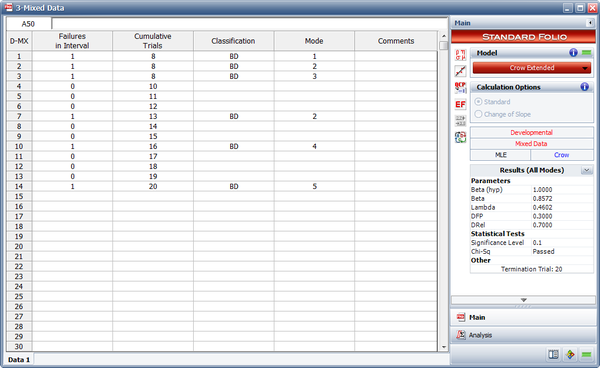
A one-shot system underwent reliability growth testing for a total of 20 trials. The test was performed as a combination of groups of units with the same configuration and individual trials. The following table shows the data set. The Failures in Interval column specifies the number of failures that occurred in each interval and the Cumulative Trials column specifies the cumulative number of trials at the end of that interval. In other words, the first three rows contain the data from the first trial, in which 8 units with the same configuration were tested and 3 failures (with different failure modes) were observed. The next row contains data from the second trial, in which 2 units with the same configuration were tested and no failures occurred. And so on.
| Mixed Data | |||
| Failures in Interval | Cumulative Trials | Classification | Mode |
|---|---|---|---|
| 1 | 8 | BD | 1 |
| 1 | 8 | BD | 2 |
| 1 | 8 | BD | 3 |
| 0 | 10 | ||
| 0 | 11 | ||
| 0 | 12 | ||
| 1 | 13 | BD | 2 |
| 0 | 14 | ||
| 0 | 15 | ||
| 1 | 16 | BD | 4 |
| 0 | 17 | ||
| 0 | 18 | ||
| 0 | 19 | ||
| 1 | 20 | BD | 5 |
The table also gives the classifications of the failure modes. There are 5 BD modes. The average effectiveness factor for the BD modes is 0.7. Do the following:
- Calculate the demonstrated reliability at the end of the test.
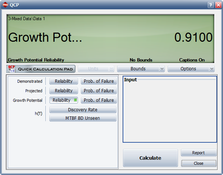
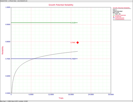
- Calculate the growth potential reliability.
Solution
-
Based on the equations presented in Crow-AMSAA (NHPP), the parameters of the Crow-AMSAA (NHPP) model are estimated as follows:
- [math]\displaystyle{ \widehat{\beta }=0.8572\,\! }[/math]
- [math]\displaystyle{ \widehat{\lambda }=0.4602\,\! }[/math]
- [math]\displaystyle{ \hat{\lambda }=\frac{n}{T_{n}^{\hat{\beta }}}\,\! }[/math]
- [math]\displaystyle{ \begin{align} \hat{\lambda }= & \frac{n}{{{T}_{n}}} \\ = & \frac{6}{20} \\ = & 0.3 \end{align}\,\! }[/math]
- [math]\displaystyle{ \begin{align} {{\lambda }_{i}}(T)=\lambda \beta {{T}^{\beta -1}},\text{with }T\gt 0,\text{ }\lambda \gt 0\text{ and }\beta \gt 0 \end{align}\,\! }[/math]
- [math]\displaystyle{ {{Q}_{i}}(20)=\widehat{\lambda }=0.3\,\! }[/math]
- [math]\displaystyle{ \begin{align} {{R}_{i}}(20)= & 1-{{Q}_{i}}(20) \\ = & 1-0.3 \\ = & 0.7 \end{align}\,\! }[/math]
- The growth potential unreliability is:
- [math]\displaystyle{ \begin{align} {{\widehat{Q}}_{GP}}(T)= & \left( \frac{{{N}_{A}}}{T}+\underset{i=1}{\overset{M}{\mathop \sum }}\,(1-{{d}_{i}})\frac{{{N}_{i}}}{T} \right) \\ = & \underset{i=1}{\overset{M}{\mathop \sum }}\,(1-0.7)\frac{{{N}_{i}}}{T} \\ = & 0.3*(\frac{1+1+1+1+1+1)}{20} \\ = & 0.09 \end{align}\,\! }[/math]
- [math]\displaystyle{ \begin{align} {{\widehat{R}}_{GP}}(T) = & 1-{{\widehat{Q}}_{GP}}(T) \\ = & 1-0.09 \\ = & 0.91 \end{align}\,\! }[/math]


Multiple Systems with Event Codes
The Multiple Systems with Event Codes data type is used to analyze the failure data from a reliability growth test in which a number of systems are tested concurrently and the implemented fixes are tracked during the test phase. With this data type, all of the systems under test are assumed to have the same system hours at any given time. The Crow Extended model is used for this data type, so all the underlying assumptions regarding the Crow Extended model apply. As such, this data type is applicable only to data from within a single test phase.
As previously presented, the failure mode classifications for the Crow Extended model are defined as follows:
- A indicates that no corrective action was performed or will be performed (management chooses not to address for technical, financial or other reasons).
- BC indicates that the corrective action was implemented during the test. The analysis assumes that the effect of the corrective action was experienced during the test (as with other test-fix-test reliability growth analyses).
- BD indicates that the corrective action will be delayed until after the completion of the current test.
Therefore, implemented fixes can be applied only to BC modes since all BD modes are assumed to be delayed until the end of the test. For each BC mode, there must be a separate entry in the data set that records the time when the fix was implemented during the test.
Event Codes
A Multiple Systems with Event Codes data sheet that is analyzed with the Crow Extended model has an Event column that allows you to indicate the types of events that occurred during a test phase. The possible event codes that can be used in the analysis are:
- I: denotes that a certain BC failure mode has been corrected at the specific time; in other words, a fix has been implemented. For this data type, each BC mode must have an associated I event. The I event is essentially a timestamp for when the fix was implemented during the test.
- Q: indicates that the failure was due to a quality issue. An example of this might be a failure caused by a bolt not being tightened down properly. You have the option to decide whether or not to include quality issues in the analysis. This option can be specified by checking or clearing the Include Q Events check box under Event Code Options on the Analysis tab.
- P: indicates that the failure was due to a performance issue. You can determine whether or not to include performance issues in the analysis. This option can be specified by checking or clearing the Include P Events check box under Event Code Options on the Analysis tab.
- X: indicates that you wish to exclude the data point from the analysis. An X can be placed in front of any existing event code (e.g., XF to exclude a particular failure time) or entered by itself. The row of data with the X will not be included in the analysis.
- S: indicates the system start time. This event code is only selectable in the Normal View.
- F: indicates a failure time.
- E: indicates the system end time. This event code is only selectable in the Normal View.
The analysis is based on the equivalent system that combines the operating hours of all the systems.
Equivalent Single System
In order to analyze a Multiple Systems with Event Codes data sheet, the data are converted into a Crow Extended equivalent single system. The implemented fixes (I events) are taken into account when building the equivalent single system from the data for multiple systems.
The basic assumptions and constraints for the use of this data type are listed below:
- Failure modes are assumed to be independent of each other and with respect to the system configuration. The same applies to their related implemented fixes (I events). As such, each mode and its related implemented fixes (I events) are examined separately in terms of their impact to the system configuration.
- If there are BC modes in the data set, there must be at least 3 unique BC modes to analyze the data (together with implemented fixes for each one of them).
- If there are BD modes in the data set, there must be at least 3 unique BD modes to analyze the data.
- To be consistent with the definition of BC modes in the Crow Extended model, every BC mode must have at least one implemented fix (I event) on at least one system.
- Implemented fixes (I events) cannot be delayed to a later phase, because the Crow Extended model applies to a single phase only.
The following list shows the basic rules for calculating the equivalent single system on which the Crow Extended model is applied. Note that the list is not exhaustive since there is an infinite number of scenarios that can occur. These rules cover the most common scenarios. The main concept is to add the time that each system was tested under the same configuration.
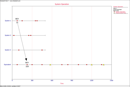
- To get to the equivalent single system, each failure time for A modes and BD modes is calculated by adding the time that each system was tested under the same configuration. In practice this means multiplying the failure time in the system by the number of total systems under test. For example, if we have 4 total systems, and system 2 has a BD1 mode at time 30, the BD1 mode failure time in the equivalent single system would be [math]\displaystyle{ 30*4=120\,\! }[/math]. If system 3 had another BD1 mode at time 40, then that would yield another BD1 mode in the equivalent single system at time [math]\displaystyle{ 40*4=160\,\! }[/math]. These calculations are done assuming that the start time for the systems are at time zero. If the start time is different than zero, then that time would have to be subtracted from the failure time on each system. For example, if system 1 started at time S=10, and there was a failure at time 30, the equivalent system time would be [math]\displaystyle{ (30-10)*4=80\,\! }[/math].
- Each failure time for a BC mode that occurred before an implemented fix (I event) for that mode is also calculated by multiplying the failure time in the system by the number of total systems in test, as described above.
- The implemented fix (I event) time in the equivalent single system is calculated by adding the test time invested in each system before that I event takes place. It is the total time that the system has spent at the same configuration in terms of that specific mode.
- If the same BC mode occurs in another system after a fix (I event) has been implemented in one or more systems, the failure time in the equivalent single system is calculated by adding the test time for that BC mode, and one of the following for each of the other systems:
- If a BC mode occurs in a system that has already seen an I event for that mode, then you add the time up to the I event.
- or
- If the I events occurred later than the BC failure time or those systems did not have any I events for that mode, then you add the time of the BC failure.
- If the same BC mode occurs in the same system after a fix (I event) has been implemented in one or more systems, the failure time in the equivalent single system is calculated by adding the test time of each system after that I event was implemented to the I event time in the equivalent single system, or zero if an I event was not present in that system.
Example: Equivalent Single System
Consider the data set shown in the following figure.

Solution
The first step to creating the equivalent system is to isolate each failure mode and its implemented fixes independently from each other. The numbered steps follow the five rules and are presented in the same numbering sequence.
- The next figure illustrates the application of rule #1 for mode BD1. The mode in the equivalent single system is calculated as [math]\displaystyle{ (75+75+75)=225\,\! }[/math] or [math]\displaystyle{ 75*3=225.\,\! }[/math]
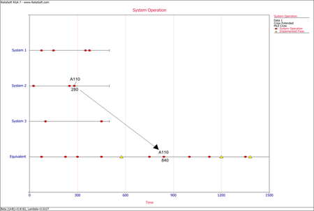
The next figure illustrates the application of rule #1 for mode A110. The mode in the equivalent single system is calculated as [math]\displaystyle{ (280+280+280)=840\,\! }[/math] or [math]\displaystyle{ 280*3=840.\,\! }[/math]
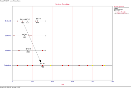
- The next figure illustrates the application of rule #2 for the first occurrence of the mode BC10 in system 1. The mode in the equivalent single system is calculated as [math]\displaystyle{ (150+150+150)=450\,\! }[/math] or [math]\displaystyle{ 150*3=450.\,\! }[/math]
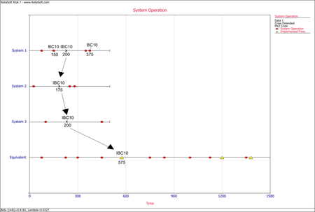
- The next figure illustrates the application of rule #3 for implemented fixes (I events) of the mode BC10. In the graph, the I events are symbolized by having the letter "I" before the naming of the mode. In this case, IBC10 is for the implemented fix of mode BC10. The IBC10 in the equivalent single system is calculated as [math]\displaystyle{ (200+175+200)=575\,\! }[/math].
- The next figure illustrates the application of rule #4 for the mode BC20 in system 1, which occurs after a fix for the same mode was implemented in system 2. The mode in the equivalent single system is calculated as [math]\displaystyle{ (350+300+350)=1000.\,\! }[/math]
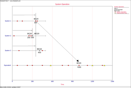
- The next figure illustrates the application of rule #5 for the second occurrence of the mode BC10 in system 1, which occurs after an implemented fix (I event) has occurred for that mode in the same system. The mode in the equivalent single system is calculated as [math]\displaystyle{ 575+(175+200+175)=1125.\,\! }[/math]
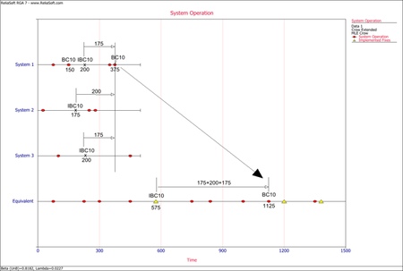
After having transferred the data set to the Crow Extended equivalent system, the data set is analyzed using the Crow Extended model. The last figure shows the growth potential MTBF plot.
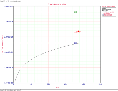


Transferring Data to an Equivalent Single System
RGA provides the capability to transfer a Multiple Systems with Event Codes data sheet to various other data types. The following picture shows the available data types that the data sheet can be converted into. When selecting to transfer to an equivalent single system, the data sheet is converted to a Crow Extended - Continuous Evaluation data sheet.

The Crow Extended - Continuous Evaluation model is designed for analyzing data across multiple test phases, while considering the data for all phases as one data set. Familiarity with this model is necessary for the discussion presented in this section.
When using the Crow Extended - Continuous Evaluation model to transfer the data sheet from Multiple Systems with Event Codes to an equivalent single system, the following rules are used (in addition to the five basic rules presented earlier for calculating the equivalent single system):
- BD modes in the Crow Extended data sheet become BD modes in the equivalent single system of the Crow Extended - Continuous Evaluation data sheet.
- BC modes in the Crow Extended data sheet become BD modes in the equivalent single system of the Crow Extended - Continuous Evaluation data sheet. These BD modes will have associated implemented fixes (I events). Implemented fixes (I events) for BC modes in the Crow Extended data sheet become implemented fixes (I events) for the converted BD modes in the equivalent single system of the Crow Extended - Continuous Evaluation data sheet.
- If an implemented fix (I event) occurred at the same time as the failure, and was implemented at that exact time across all systems, then this becomes a BC mode in the equivalent single system. If the fixes (I events) were not all implemented at the same time or if the fix was not implemented on all systems at the failure time, then this becomes a BD mode in the equivalent single system.
The next figure shows the transferred equivalent single system Crow Extended - Continuous Evaluation data sheet from the Multiple Systems with Event Codes data sheet for the data from the Equivalent Single System example given above.

Iteration Method for Naming Repeated Modes
When recording modes for transfer from the Multiple Systems with Event Codes to a Crow Extended -Continuous Evaluation equivalent single system, it is recommended to consider using an iteration method to name subsequent recurrences of the same mode. This will help alleviate any issues with the conversion of the definitions of the modes from the Crow Extended model to the Crow Extended - Continuous Evaluation model. For example, if the first occurrence of a mode is BC25, then the second occurrence is suggested to be named as BC25.1. The reasoning behind this recommendation is that in the case that BC25 in the Multiple Systems with Event Codes data sheet has received implemented fixes (I events) at the same time that the failure occurred in all systems, then this mode will be translated as a BC mode in the Crow Extended - Continuous Evaluation equivalent single system. The next recurring failure would also be treated as a BC mode, but in reality it did not have an implemented fix (I event) at the time of failure.
For example, consider the data set shown in the following figure, which represents one system only for simplicity. Notice that the modes BC25, BC35 and BC45 received implemented fixes at the time of failure. Based on that, when they get transferred to the Crow Extended - Continuous Evaluation equivalent single system, they will be considered as BC modes. The subsequent failures of the modes 25, 35 and 45 will also be converted to BC modes, when in reality they had implemented fixes (I events) at a later time.

The RGA software will display a warning if you try to convert this data sheet without using iterations.
The next figure shows the same data sheet with the use of iterations for the modes 25, 35 and 45. The subsequent failures are named as BC25.1, BC35.1 and BC45.1.

This way, the conversion to the Crow Extended - Continuous Evaluation model occurs in a valid fashion, because although the original BC modes are converted to BC25, BC35 and BC45, the subsequent failures are converted to BD25.1, BD35.1 and BD45.1 together with their respective implemented fixes (I events). This is shown in the next figure below. Note that the use of iterations is recommended only when transferring to the Crow Extended - Continuous Evaluation equivalent single system; it is not necessary when using the Multiple Systems with Event Codes data sheet that is calculated with the Crow Extended model.

More Examples
Adjusting the Failure Mode Management Strategy
Three systems were subjected to a reliability growth test to evaluate the prototype of a new product. Based on a failure analysis on the results of the test, the proposed management strategy is to delay corrective actions until after the test. The tables shown next display the data set and the associated effectiveness factors for the unique BD modes.
| Multiple Systems (Concurrent Operating Times) Data | |||
| System 1 | System 2 | System 3 | |
|---|---|---|---|
| Start Time | 0 | 0 | 0 |
| End Time | 541 | 454 | 436 |
| Times-to-Failure | 83 BD37 | 26 BD25 | 23 BD30 |
| 83 BD43 | 26 BD43 | 46 BD49 | |
| 83 BD46 | 57 BD37 | 127 BD47 | |
| 169 A45 | 64 BD19 | 166 A2 | |
| 213 A18 | 169 A45 | 169 BD23 | |
| 299 A42 | 213 A32 | 213 BD7 | |
| 375 A1 | 231 BD8 | 213 BD29 | |
| 431 BD16 | 231 BD25 | 255 BD26 | |
| 231 BD27 | 369 A33 | ||
| 231 A28 | 374 BD29 | ||
| 304 BD24 | 380 BD22 | ||
| 383 BD40 | 415 BD7 | ||
| Effectiveness factors | |
| BD Mode | Effectiveness Factor |
|---|---|
| 30 | 0.75 |
| 43 | 0.5 |
| 25 | 0.5 |
| 49 | 0.75 |
| 37 | 0.9 |
| 19 | 0.75 |
| 46 | 0.75 |
| 47 | 0.25 |
| 23 | 0.5 |
| 7 | 0.25 |
| 29 | 0.25 |
| 8 | 0.5 |
| 27 | 0.5 |
| 26 | 0.75 |
| 24 | 0.5 |
| 22 | 0.5 |
| 40 | 0.75 |
| 16 | 0.75 |
The prototype is required to meet a projected MTBF goal of 55 hours. Do the following:
- Estimate the parameters of the Crow Extended model.
- Based on the current management strategy what is the projected MTBF?
- If the projected MTBF goal is not met, alter the current management strategy to meet this requirement with as little adjustment as possible and without changing the EFs of the existing BD modes. Assume an EF = 0.7 for any newly assigned BD modes.
Solution
- The next figure shows the estimated Crow Extended parameters.
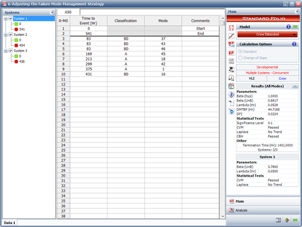
- There are a couple of ways to calculate the projected MTBF, but the easiest is via the Quick Calculation Pad (QCP). The following result shows that the projected MTBF is estimated to be 53.9390 hours, which is below the goal of 55 hours.
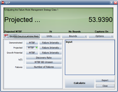
- To reach our goal, or to see if we can even get there, the management strategy must be changed. The effectiveness factors for the existing BD modes cannot be changed; however, it is possible to change an A mode to a BD mode, but which A mode(s) should be changed? To answer this question, create an Individual Mode Failure Intensity plot with just the A modes displayed, as shown next. As you can see from the plot, failure mode A45 has the highest failure intensity. Therefore, among the A modes, this particular failure mode has the greatest negative effect on the system MTBF.
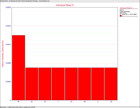
Change A45 to BD45. Be sure to change all instances of A45 to a BD mode. Enter an effectiveness factor of 0.7 for BD45, and then recalculate the parameters of the Crow Extended model. Now go back to the QCP to calculate the projected MTBF, as shown below. The projected MTBF is now estimated to be 55.5903 hours. Based on the change in the management strategy, the projected MTBF goal is now expected to be met.
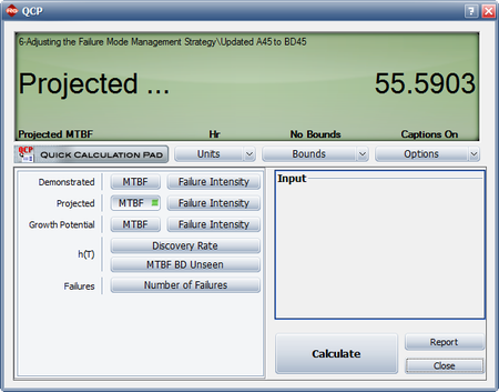


Estimating the Failure Intensity Remaining After Fixes
A reliability growth test was conducted for 200 hours. Some of the corrective actions were applied during the test while others were delayed until after the test was completed. The tables below give the data set and the effectiveness factors for the BD modes. Do the following:
- Estimate the parameters of the Crow Extended model.
- Determine the average effectiveness factor of the BC modes using the Function Wizard.
- What percent of the failure intensity will be left in the system due to the BD modes after implementing the delayed fixes?
| Grouped Failure Times Data | |||
| Number at Event | Time to Event | Classification | Mode |
|---|---|---|---|
| 3 | 25 | BC | 1 |
| 1 | 25 | BD | 9 |
| 1 | 25 | BC | 2 |
| 1 | 50 | BD | 10 |
| 1 | 50 | BD | 11 |
| 1 | 75 | BD | 12 |
| 1 | 75 | BC | 3 |
| 2 | 75 | BD | 13 |
| 1 | 75 | A | |
| 1 | 100 | BC | 4 |
| 1 | 100 | BD | 14 |
| 1 | 125 | BD | 15 |
| 1 | 125 | A | |
| 1 | 125 | A | |
| 1 | 125 | BC | 5 |
| 1 | 125 | BD | 10 |
| 1 | 125 | BC | 6 |
| 1 | 150 | A | |
| 1 | 150 | BD | 16 |
| 1 | 175 | BC | 4 |
| 1 | 175 | BC | 8 |
| 1 | 175 | A | |
| 1 | 175 | BC | 7 |
| 1 | 200 | BD | 16 |
| 1 | 200 | BC | 3 |
| 1 | 200 | BD | 17 |
| Effectiveness Factors | |
| BD Mode | Effectiveness Factor |
|---|---|
| 9 | 0.75 |
| 10 | 0.5 |
| 11 | 0.9 |
| 12 | 0.6 |
| 13 | 0.8 |
| 14 | 0.8 |
| 15 | 0.25 |
| 16 | 0.75 |
| 17 | 0.8 |
Solution
- The next figure shows the estimated parameters of the Crow Extended model.
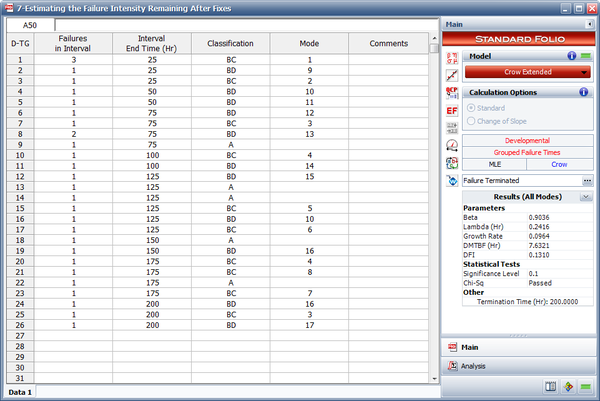
- Insert a general spreadsheet into the folio, and then access the Function Wizard. In the Function Wizard, select Average Effectiveness Factor from the list of available functions and under Avg. Eff. Factor select BC modes, as shown next. Click Insert and the result will be inserted into the general spreadsheet. The average effectiveness factor for the BC modes is 0.6983.
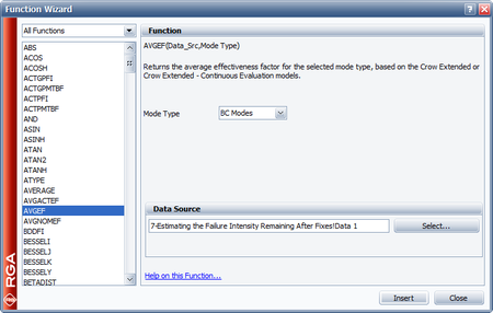
- The failure intensity left in the system due to the BD modes can be determined using the Failure Mode Strategy plot, as shown next. Therefore, the failure intensity left in the system due to the BD modes is 1.79%.
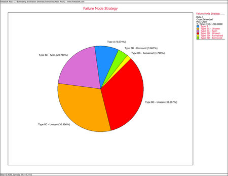


Determining if Design Will Meet MTBF Goal
Two prototypes of a new design are tested simultaneously. Whenever a failure is observed for one unit, the current operating time of the other unit is also recorded. The test is terminated after 300 hours. All of the design changes for the prototypes were delayed until after completing the test. The data set is given in the table below. Assume a fixed effectiveness factor equal to 0.7. The MTBF goal for the new design is 30 hours. Do the following:
- Estimate the parameters of the Crow Extended model.
- What is the projected MTBF and growth potential?
- Under the current management strategy, is it even possible to reach the MTBF goal of 30 hours?
| Multiple Systems (Known Operating Times) Data | ||||
| Failed Unit ID | Time Unit 1 | Time Unit 2 | Classification | Mode |
|---|---|---|---|---|
| 1 | 16.5 | 0 | BD | seal leak |
| 1 | 16.5 | 0 | BD | valve |
| 1 | 17 | 0 | A | |
| 2 | 20.5 | 0.9 | A | |
| 2 | 25.3 | 3.8 | BD | hose |
| 2 | 28.7 | 4.6 | BD | operator error |
| 1 | 41.8 | 14.7 | BD | bearing |
| 1 | 45.5 | 17.6 | A | |
| 2 | 48.6 | 22 | A | |
| 2 | 49.6 | 23.4 | BD | seal leak |
| 1 | 51.4 | 26.3 | A | |
| 1 | 58.2 | 35.7 | BD | seal leak |
| 2 | 59 | 36.5 | A | |
| 2 | 60.6 | 37.6 | BD | hose |
| 1 | 61.9 | 39.1 | BD | seal leak |
| 1 | 76.6 | 55.4 | BD | bearing |
| 2 | 81.1 | 61.1 | A | |
| 1 | 84.1 | 63.6 | A | |
| 1 | 84.7 | 64.3 | A | |
| 1 | 94.6 | 72.6 | A | |
| 2 | 100 | 78.1 | BD | valve |
| 1 | 104 | 81.4 | BD | bearing |
| 2 | 104.8 | 85.9 | BD | spring |
| 2 | 105.9 | 87.1 | BD | operator error |
| 1 | 108.8 | 89.9 | BD | hose |
| 2 | 132.4 | 119.5 | BD | spring |
| 2 | 132.4 | 150.1 | BD | operator error |
| 2 | 132.4 | 153.7 | A | |
Solution
- The next figure shows the estimated Crow Extended parameters.
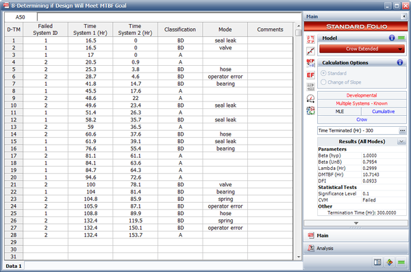
- One possible method for calculating the projected MTBF and growth potential is to use the Quick Calculation Pad, but you can also view these two values at the same time by viewing the Growth Potential MTBF plot, as shown next. From the plot, the projected MTBF is equal to 16.87 hours and the growth potential is equal to 18.63 hours.
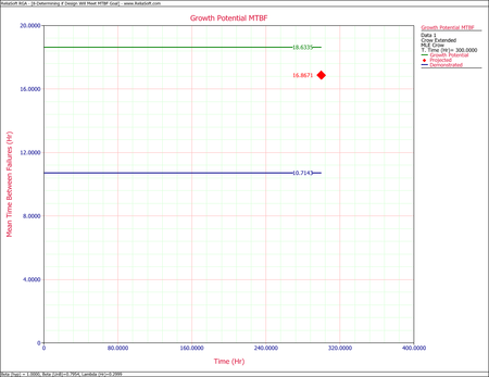
- The current projected MTBF and growth potential MTBF are both well below the required goal of 30 hours. To check if this goal can even be reached, you can set the effectiveness factor equal to 1. In other words, if all of the corrective actions were to remove the failure modes completely, what would be the projected and growth potential MTBF?
Change the fixed effectiveness factor to 1, then recalculate the parameters and refresh the Growth Potential plot, as shown next. Even if you assume an effectiveness factor equal to 1, the growth potential is still only 27.27 hours. Based on the current design process, it will not be possible to reach the MTBF goal of 30 hours. Therefore, you have two options: start a new design stage or reduce the required MTBF goal.