Template:Reliability growth planning rga

Reliability Growth Planning

Background

In developmental reliability growth testing, the objective is to test a system, find problem failure modes, at some point incorporate corrective actions, and therefore increase the reliability of the system. This process is continued for the duration of the test time. If the corrective actions are effective then the system Mean Time Between Failures (MTBF) will move from an initial low value to a higher value. Typically the objective of reliability growth testing is not to just increase the MTBF, but to increase it to a particular value. In other words, increase the MTBF to meet a goal or requirement. Therefore, determining how much test time is needed for a particular system is generally always of interest in reliability growth testing. This brings us to the topic of growth planning.

In this chapter, we will address the common questions engineers and managers face at the planning stage of product development, in terms of meeting the design reliability goals. Planning for required test time, setting realistic reliability goals and creating a strategy for meeting those goals are all essential parts of project management. It is therefore necessary to have a tool that can be utilized for such planning purposes. The basis of the tool will be the Duane Postulate and a model will be developed which incorporates the realities faced during development and generates a plan that can be used as a guideline during developmental testing. The Duane Postulate is based on empirical observations and reflects a learning curve pattern for reliability growth. This identical learning curve pattern forms the basis of the Crow-AMSAA (NHPP) model. The Duane Postulate is also reflected in the Crow Extended model in the form of the discovery function [math]\displaystyle{ h(t) }[/math] .

The discovery function is the rate in which new, distinct problems are being discovered during reliability growth development testing. The Crow-AMSAA (NHPP) model is a special case of the discovery function. Consider that when a new, distinct failure mode is first seen the testing is stopped and a corrective action is incorporated before the testing is resumed. In addition, suppose that the corrective action is highly effective so that the failure mode is unlikely to be seen again. In this case, the only failures observed during the reliability growth test are first occurrences of failure modes. Therefore, if the Crow-AMSAA (NHPP) model and the Duane Postulate are accepted as the pattern for a test-fix-test reliability growth testing program, then the form of the Crow-AMSAA (NHPP) model must be the form for the discovery function, [math]\displaystyle{ h(t) }[/math] .

To be consistent with the Duane Postulate and the Crow-AMSAA (NHPP) model the discovery function must be of the same form. This form of the discovery function is an important property of the Crow Extended model and its application in growth planning. As with the Crow-AMSAA (NHPP) model, this form of the discovery function ties the model directly to real-world data and experiences The use of the Duane Postulate as a reliability growth planning model poses two significant drawbacks:The first drawback is that the Duane Postulate's MTBF is zero at time equal to zero. This was addressed in MIL-HDBK-189 by specifying a time [math]\displaystyle{ {{T}_{i}} }[/math] where growth starts after [math]\displaystyle{ {{T}_{i}} }[/math] and the Duane Postulate applies [13]. However, determining [math]\displaystyle{ {{T}_{i}} }[/math] is subjective and is not a desirable property of MIL-HDBK-189. The second drawback is that the MTBF for the Duane Postulate increases indefinitely to infinity, which is not realistic.

Therefore a desirable feature of a planning model is that:

1) The discovery function must have the form of the Crow-AMSAA (NHPP) model and the Duane Postulate.

2) The start time [math]\displaystyle{ {{T}_{i}} }[/math] is not required as an input.

3) An upper bound on the system MTBF is specified in the model.

All of these desirable features are included in the planning model discussed in this chapter, which is based on the Crow Extended model.

Introduction

In developmental reliability growth testing, the objective is to test a system, find problem failure modes, incorporate corrective actions and therefore increase the reliability of the system. This process is continued for the duration of the test time. If the corrective actions are effective then the system mean time between failures (MTBF) or mean trials between failures (MTrBF) will move from an initial low value to a higher value. Typically, the objective of reliability growth testing is not to just increase the MTBF/MTrBF, but to increase it to a particular value called the goal or requirement. Therefore, determining how much test time is needed for a particular system is generally of particular interest in reliability growth testing.

The Duane postulate is based on empirical observations, and it reflects a learning curve pattern for reliability growth. This learning curve pattern forms the basis of the Crow-AMSAA (NHPP) model. The Duane postulate is also reflected in the Crow Extended model in the form of the discovery function [math]\displaystyle{ h(t)\,\! }[/math].

The discovery function is the rate in which new, distinct problems are being discovered during reliability growth development testing. The Crow-AMSAA (NHPP) model is a special case of the discovery function. Consider that when a new and distinct failure mode is first seen, the testing is stopped and a corrective action is incorporated before the testing is resumed. In addition, suppose that the corrective action is highly effective that the failure mode is unlikely to be seen again. In this case, the only failures observed during the reliability growth test are the first occurrences of the failure modes. Therefore, if the Crow-AMSAA (NHPP) model and the Duane postulate are accepted as the pattern for a test-fix-test reliability growth testing program, then the form of the Crow-AMSAA (NHPP) model must be the form for the discovery function, [math]\displaystyle{ h(t)\,\! }[/math].

To be consistent with the Duane postulate and the Crow-AMSAA (NHPP) model, the discovery function must be of the same form. This form of the discovery function is an important property of the Crow extended model and its application in growth planning. As with the Crow-AMSAA (NHPP) model, this form of the discovery function ties the model directly to real-world data and experiences.

Growth Planning Models

There are two types of reliability growth planning models available in RGA:

• Continuous Reliability Growth Planning

• Discrete Reliability Growth Planning

Growth Planning Inputs

The following parameters are used in both the continuous and discrete reliability growth models.

Management Strategy Ratio & Initial Failure Intensity

When a system is tested and failure modes are observed, management can make one of two possible decisions, either to fix or to not fix the failure mode. Therefore, the management strategy places failure modes into two categories: A modes and B modes. The A modes are all failure modes such that, when seen during the test, no corrective action will be taken. This accounts for all modes for which management determines to be not economical or otherwise justified to take a corrective action. The B modes are either corrected during the test or the corrective action is delayed to a later time. The management strategy is defined by what portion of the failures will be fixed.

Let [math]\displaystyle{ {{\lambda }_{I}}\,\! }[/math] be the initial failure intensity of the system in test. [math]\displaystyle{ {{\lambda }_{A}}\,\! }[/math] is defined as the A mode's initial failure intensity and [math]\displaystyle{ {{\lambda }_{B}}\,\! }[/math] is defined as the B mode's initial failure intensity. [math]\displaystyle{ {{\lambda }_{A}}\,\! }[/math] is the failure intensity of the system that will not be addressed by corrective actions even if a failure mode is seen during testing. [math]\displaystyle{ {{\lambda }_{B}}\,\! }[/math] is the failure intensity of the system that will be addressed by corrective actions if a failure mode is seen during testing.

Then, the initial failure intensity of the system is:

[math]\displaystyle{ \begin{align} {{\lambda }_{I}}={{\lambda }_{A}}+{{\lambda }_{B}} \end{align}\,\! }[/math]

The initial system MTBF is:

[math]\displaystyle{ {{M}_{I}}=\frac{1}{{{\lambda }_{I}}}\,\! }[/math]

Based on the initial failure intensity definitions, the management strategy ratio is defined as:

[math]\displaystyle{ msr=\frac{{{\lambda }_{B}}}{{{\lambda }_{A}}+{{\lambda }_{B}}}\,\! }[/math]

The [math]\displaystyle{ msr\,\! }[/math] is the portion of the initial system failure intensity that will be addressed by corrective actions, if seen during the test.

The failure mode intensities of the type A and type B modes are:

[math]\displaystyle{ \begin{align} {{\lambda }_{A}}= & \left( 1-msr \right)\cdot {{\lambda }_{I}} \\ {{\lambda }_{B}}= & msr\cdot {{\lambda }_{I}} \end{align}\,\! }[/math]

Effectiveness Factor

When a delayed corrective action is implemented for a type B failure mode, in other words a BD mode, the failure intensity for that mode is reduced if the corrective action is effective. Once a BD mode is discovered, it is rarely totally eliminated by a corrective action. After a BD mode has been found and fixed, a certain percentage of the failure intensity will be removed, but a certain percentage of the failure intensity will generally remain. The fraction decrease in the BD mode failure intensity due to corrective actions, [math]\displaystyle{ d\,\! }[/math], [math]\displaystyle{ \left( 0\lt d\lt 1 \right),\,\! }[/math] is called the effectiveness factor (EF).

A study on EFs showed that an average EF, [math]\displaystyle{ d\,\! }[/math], is about 70%. Therefore, about 30% (i.e., [math]\displaystyle{ 100(1-d)%\,\! }[/math]) of the BD mode failure intensity will typically remain in the system after all of the corrective actions have been implemented. However, individual EFs for the failure modes may be larger or smaller than the average. This average value of 70% can be used for planning purposes, or if such information is recorded, an average effectiveness factor from a previous reliability growth program can be used.

MTBF Goal

When putting together a reliability growth plan, a goal MTBF/MTrBF [math]\displaystyle{ {{M}_{G}}\,\! }[/math] (or goal failure intensity [math]\displaystyle{ {{\lambda }_{G}}\,\! }[/math] ) is defined as the requirement or target for the product at the end of the growth program.

Growth Potential

The failure intensity remaining in the system at the end of the test will depend on the management strategy given by the classification of the type A and type B failure modes. The engineering effort applied to the corrective actions determines the effectiveness factors. In addition, the failure intensity depends on [math]\displaystyle{ h(t)\,\! }[/math], which is the rate at which problem failure modes are being discovered during testing. The rate of discovery drives the opportunity to take corrective actions based on the seen failure modes, and it is an important factor in the overall reliability growth rate. The reliability growth potential is the limiting value of the failure intensity as time [math]\displaystyle{ T\,\! }[/math] increases. This limit is the maximum MTBF that can be attained with the current management strategy. The maximum MTBF/MTrBF will be attained when all type B modes have been observed and fixed.

If all the discovered type B modes are corrected by time [math]\displaystyle{ T\,\! }[/math], that is, no deferred corrective actions at time [math]\displaystyle{ T\,\! }[/math], then the growth potential is the maximum attainable with the type B designation of the failure modes and the corresponding assigned effectiveness factors. This is called the nominal growth potential. In other words, the nominal growth potential is the maximum attainable growth potential assuming corrective actions are implemented for every mode that is planned to be fixed. In reality, some corrective actions might be implemented at a later time due to schedule, budget, engineering, etc.

If some of the discovered type B modes are not corrected at the end of the current test phase, then the prevailing growth potential is below the maximum attainable with the type B designation of the failure modes and the corresponding assigned effectiveness factors.

If all type B failure modes are discovered and corrected with an average effectiveness factor, [math]\displaystyle{ d\,\! }[/math], then the maximum reduction in the initial system failure intensity is the growth potential failure intensity:

[math]\displaystyle{ {{\lambda }_{GP}}={{\lambda }_{A}}+\left( 1-d \right){{\lambda }_{B}}\,\! }[/math]

The growth potential MTBF/MTrBF is:

[math]\displaystyle{ {{M}_{GP}}=\frac{1}{{{\lambda }_{GP}}}\,\! }[/math]

Note that based on the equations for the initial failure intensity and the management strategy ratio (given in the Management Strategy and Initial Failure Intensity section), the initial failure intensity is equal to:

[math]\displaystyle{ {{\lambda }_{I}}=\frac{{{\lambda }_{GP}}}{1-d\cdot msr}\,\! }[/math]

Growth Potential Design Margin

The Growth Potential Design Margin ( [math]\displaystyle{ GPDM\,\! }[/math] ) can be considered as a safety margin when setting target MTBF/MTrBF values for the reliability growth plan. It is common for systems to degrade in terms of reliability when a prototype product is going into full manufacturing. This is due to variations in materials, processes, etc. Furthermore, the in-house reliability growth testing usually overestimates the actual product reliability because the field usage conditions may not be perfectly simulated during testing. Typical values for the [math]\displaystyle{ GPDM\,\! }[/math] are around 1.2. Higher values yield less risk for the program, but require a more rigorous reliability growth test plan. Lower values imply higher program risk, with less safety margin.

During the planning stage, the growth potential MTBF/MTrBF, [math]\displaystyle{ {{M}_{GP}},\,\! }[/math] can be calculated based on the goal MTBF, [math]\displaystyle{ {{M}_{G}},\,\! }[/math] and the growth potential design margin, [math]\displaystyle{ GPDM\,\! }[/math].

[math]\displaystyle{ {{M}_{GP}}=GPDM\cdot {{M}_{G}}\,\! }[/math]

or in terms of failure intensity:

[math]\displaystyle{ {{\lambda }_{GP}}=\frac{{{\lambda }_{G}}}{GPDM}\,\! }[/math]

Reliability Growth Planning Examples

Example 1

A complex system is under design. The reliability team wants to create an overall reliability growth plan based on the Crow Extended model. The inputs to the model are the following:

• The requirement or goal MTBF is [math]\displaystyle{ {{M}_{G}}=56 }[/math] hours.

• The Growth Potential Design Margin Factor is [math]\displaystyle{ GPDM=1.35 }[/math] .

• The Average Effectiveness Factor is [math]\displaystyle{ d\quad =0.7. }[/math]

• The Management Strategy is [math]\displaystyle{ msr=0.95 }[/math] .

• The beta parameter for the discovery function, [math]\displaystyle{ h\left( t \right), }[/math] of the Type B failure modes is [math]\displaystyle{ \beta =0.7. }[/math]

• The test will be conducted in three phases. The cumulative phase end times are [math]\displaystyle{ {{T}_{1}}=1500,{{T}_{2}}=3500 }[/math] and [math]\displaystyle{ {{T}_{3}}=4500 }[/math] hours. The average fix delays for each phase are and [math]\displaystyle{ {{L}_{3}}=1000 }[/math] test hours, respectively.

Find the following:

1) The growth potential MTBF and failure intensity.

2) The initial failure intensity.

3) The Type A and Type B initial failure intensity.

4) The parameter [math]\displaystyle{ \lambda }[/math] of the Crow Extended model.

5) The Type B failure mode discovery function.

6) The initialization time, [math]\displaystyle{ {{t}_{0}}, }[/math] for the nominal failure intensity function.

7) The nominal idealized failure intensity function.

8) The nominal time to reach the MTBF goal.

9) The MTBF that can be reached at the end of the last test phase based on the nominal idealized growth curve.

10) The actual initialization time for Phase 1, [math]\displaystyle{ T_{0}^{AIC}. }[/math]

11) The MTBF that can be reached at the end of the last test phase based on the actual idealized growth curve.

12) The actual time to reach the MTBF goal.

13) The actual time to reach the MTBF goal if the cumulative end phase time for the third (last) phase is [math]\displaystyle{ {{T}_{3}}=6000 }[/math] hours.

14) Use RGA 7 to generate the results for this example. Consider the cumulative last phase as [math]\displaystyle{ {{T}_{3}}=6000 }[/math] hours, as given in question 13.

Solution

1) Based on Eqn. (MP), the growth potential MTBF is:

[math]\displaystyle{ \begin{align} & {{M}_{GP}}= & 56\cdot 1.35 \\ & = & 75.6 \end{align} }[/math]

From Eqn. (lambda GP), the growth potential failure intensity is:

[math]\displaystyle{ \begin{align} & {{\lambda }_{GP}}= & \frac{1}{{{M}_{GP}}} \\ & = & \frac{1}{75.6} \\ & = & 0.0132 \end{align} }[/math]

2) The initial failure intensity is given by Eqn. (lambda):

[math]\displaystyle{ \begin{align} & {{\lambda }_{I}}= & \frac{{{\lambda }_{GP}}}{1-d\cdot msr} \\ & = & \frac{0.0132}{\left( 1-0.7\cdot 0.95 \right)} \\ & = & 0.0394 \end{align} }[/math]

3) From Eqn. (lambda), the Type A failure mode intensity, [math]\displaystyle{ {{\lambda }_{A}}, }[/math] is:

From Eqn. (Lambda), the Type B failure mode intensity, [math]\displaystyle{ {{\lambda }_{B}}, }[/math] is:

[math]\displaystyle{ \begin{align} & {{\lambda }_{B}}= & msr\cdot {{\lambda }_{I}} \\ & = & 0.95\cdot 0.0394 \\ & = & 0.0375 \end{align} }[/math]

4) Using the inputs of [math]\displaystyle{ {{\lambda }_{B}} }[/math] and [math]\displaystyle{ \beta }[/math] in Eqn. (lambdaithamma) we have:

[math]\displaystyle{ 0.0375=\frac{{{\lambda }^{\left( \tfrac{1}{0.7} \right)}}}{\Gamma \left( 1+\tfrac{1}{0.7} \right)} }[/math]

or:

[math]\displaystyle{ 0.0375=\frac{{{\lambda }^{1.428}}}{1.2658} }[/math]

or:

[math]\displaystyle{ \begin{align} & \lambda = & {{\left( 0.0375\cdot 1.2658 \right)}^{\left( \tfrac{1}{1.428} \right)}} \\ & = & 0.1184 \end{align} }[/math]

5) The Type B failure mode discovery function is:

[math]\displaystyle{ h\left( t \right)=\lambda \beta {{t}^{\beta -1}} }[/math]

Since we know the [math]\displaystyle{ \lambda }[/math] and [math]\displaystyle{ \beta }[/math] parameters, we have:

[math]\displaystyle{ \begin{align} & h\left( t \right)= & 0.1183\cdot 0.7{{t}^{0.7-1}} \\ & = & 0.0828{{t}^{-0.3}} \end{align} }[/math]

6) Based on Eqn. (initilization time), the initialization time, [math]\displaystyle{ {{t}_{0}}, }[/math] is:

[math]\displaystyle{ \begin{align} & {{t}_{0}}= & {{\left[ \frac{{{\lambda }_{I}}-{{\lambda }_{A}}-(1-d){{\lambda }_{B}}}{d\lambda \beta } \right]}^{\tfrac{1}{\beta -1}}} \\ & = & {{\left[ \frac{0.0394-0.001974-(1-0.7)0.0375}{0.7\cdot 0.1183\cdot 0.7} \right]}^{\tfrac{1}{0.7-1}}} \end{align} }[/math]

or:

[math]\displaystyle{ {{t}_{0}}=14.07 }[/math]

7) Based on Eqns. (Nominal FI) and (Nominal FI for time less than t0), the nominal idealized growth curve is given by the following equation:

[math]\displaystyle{ {{r}_{NI}}\left( t \right)=\left\{ \begin{matrix} {{\lambda }_{I}} & t\le {{t}_{0}} \\ \begin{matrix} {{r}_{IT}}(t)={{\lambda }_{A}}+(1-d){{\lambda }_{B}}+d\lambda \beta {{t}^{\left( \beta -1 \right)}} \\ \end{matrix} & t\gt {{t}_{0}} \\ \end{matrix} \right\} }[/math]

or:

[math]\displaystyle{ {{r}_{NI}}\left( t \right)=\left\{ \begin{matrix} 0.0394 & t\le 14.07 \\ =0.0013+0.058\cdot {{t}^{-0.3}} & t\gt 14.07 \\ \end{matrix} \right\} }[/math]

8) Based on Eqn. (tgoalominal), the nominal time to reach the MTBF goal is:

[math]\displaystyle{ {{t}_{N,goal}}={{\left[ \frac{{{r}_{G}}-{{\lambda }_{A}}-(1-d){{\lambda }_{B}}}{d\lambda \beta } \right]}^{\tfrac{1}{\beta -1}}} }[/math]

For the goal failure intensity we have:

[math]\displaystyle{ \begin{align} & {{r}_{G}}= & \frac{1}{{{M}_{G}}} \\ & = & \frac{1}{56} \\ & = & 0.01785 \end{align} }[/math]

So the nominal time to reach the MTBF goal is:

[math]\displaystyle{ \begin{align} & {{t}_{N,G}}= & {{\left[ \frac{0.01785-0.001974-(1-0.7)0.0375}{0.7\cdot 0.1184\cdot 0.7} \right]}^{^{\tfrac{1}{\beta -1}}}} \\ & = & 4578\text{ hours} \end{align} }[/math]

9) Using Eqn. (Nominal FI) we find the failure intensity that can be reached at the end of the last test phase based on the nominal idealized growth curve, [math]\displaystyle{ {{r}_{NI,final}} }[/math] . The total (cumulative) test time is [math]\displaystyle{ T=4500 }[/math] hours. Therefore we have:

[math]\displaystyle{ \begin{align} & {{r}_{NI,final}}= & {{\lambda }_{A}}+(1-d){{\lambda }_{B}}+d\lambda \beta {{T}^{\left( \beta -1 \right)}}\text{ } \\ & = & 0.0019+\left( 1-0.7 \right)0.0375+0.7\cdot 0.1184\cdot 0.7\cdot {{(4500)}^{0.7-1}} \\ & = & 0.01788 \end{align} }[/math]

So the nominal final MTBF that can be reached at 4500 hours of test time is:

[math]\displaystyle{ \begin{align} & {{M}_{NI,final}}= & \frac{1}{{{r}_{NI,final}}} \\ & = & \frac{1}{0.01788} \\ & = & 55.92 \end{align} }[/math]

10) We can find the actual initialization time by using Eqn. (actualnitilizationime):

[math]\displaystyle{ T_{0}^{AIC}=\frac{{{t}_{0}}}{\left( \tfrac{{{T}_{1}}-{{L}_{1}}}{{{T}_{1}}} \right)} }[/math]

For question 6, we had found that [math]\displaystyle{ {{t}_{0}}=14.07 }[/math] . So we have:

[math]\displaystyle{ \begin{align} & T_{0}^{AIC}= & \frac{14.07}{\left( \tfrac{1500-500}{1500} \right)} \\ & = & 21.10887 \end{align} }[/math]

11) The failure intensity that can be reached at the end of the last test phase based on the actual idealized growth curve is given by Eqn. (ActIhase) for [math]\displaystyle{ T=4500 }[/math] hours:

[math]\displaystyle{ \begin{align} & {{r}_{AI,final}}(T)= & {{\lambda }_{A}}+(1-d){{\lambda }_{B}} \\ & & +d\lambda \beta {{\left[ {{T}_{2}}-{{L}_{2}}+\left( \frac{{{T}_{3}}-{{L}_{3}}-{{T}_{2}}+{{L}_{2}}}{{{T}_{3}}-{{T}_{2}}} \right)(T-{{T}_{2}}) \right]}^{(\beta -1)}} \end{align} }[/math]

Therefore:

[math]\displaystyle{ \begin{align} & {{r}_{AI,final}}(T)= & 0.0019+\left( 1-0.7 \right)0.0375+0.7\cdot 0.1184\cdot 0.7 \\ & & \cdot {{\left[ 3500-700+\left( \frac{4500-1000-3500+700}{4500-3500} \right)(4500-3500) \right]}^{(0.7-1)}} \end{align} }[/math]

Therefore:

[math]\displaystyle{ {{r}_{AI,final}}(T)=0.0182 }[/math]

So the actual final MTBF that can be reached at 4500 hours of test time is:

[math]\displaystyle{ \begin{align} & {{M}_{AI,final}}= & \frac{1}{{{r}_{AI,final}}} \\ & = & \frac{1}{0.0182} \\ & = & 54.80 \end{align} }[/math]

12) From question 11, it is shown that the actual final MTBF that can be reached at 4500 hours of test time is less than the MTBF goal for the program. So, in accordance with the third case that is described in Section 11.2.4.3, this is the scenario where the actual time to meet the MTBF goal will not be calculated since the reliability growth program needs to be redesigned.

13) The failure intensity that can be reached at the end of the last test phase based on the actual idealized growth curve is given by Eqn. (ActIhase) for [math]\displaystyle{ T={{T}_{3}}=6000 }[/math] hours:

[math]\displaystyle{ \begin{align} & {{r}_{AI,final}}(T)= & {{\lambda }_{A}}+(1-d){{\lambda }_{B}} \\ & & +d\lambda \beta {{\left[ {{T}_{2}}-{{L}_{2}}+\left( \frac{{{T}_{3}}-{{L}_{3}}-{{T}_{2}}+{{L}_{2}}}{{{T}_{3}}-{{T}_{2}}} \right)(T-{{T}_{2}}) \right]}^{(\beta -1)}} \end{align} }[/math]

Therefore:

[math]\displaystyle{ \begin{align} & {{r}_{AI,final}}(T)= & 0.0019+\left( 1-0.7 \right)0.0375+0.7\cdot 0.1184\cdot 0.7 \\ & & \cdot {{\left[ 3500-700+\left( \frac{6000-1000-3500+700}{6000-3500} \right)(6000-3500) \right]}^{(0.7-1)}} \end{align} }[/math]

Therefore:

[math]\displaystyle{ {{r}_{AI,final}}(T)=0.0177 }[/math]

So, the actual final MTBF that can be reached at 6000 hours of test time is:

[math]\displaystyle{ \begin{align} & {{M}_{AI,final}}= & \frac{1}{{{r}_{AI,final}}} \\ & = & \frac{1}{0.0177} \\ & = & 56.38 \end{align} }[/math]

In this case, the actual MTBF goal becomes higher than the target MTBF sometime during the last phase. Using Eqn. (toalctual), we can determine the actual time to reach the MTBF goal:

[math]\displaystyle{ {{t}_{AC,G}}=\frac{{{t}_{N,G}}-{{T}_{F-1}}+{{L}_{F-1}}}{\left( \tfrac{{{T}_{F}}-{{L}_{F}}-{{T}_{F-1}}+{{L}_{F-1}}}{{{T}_{F}}-{{T}_{F-1}}} \right)}+{{T}_{F-1}} }[/math]

Therefore:

[math]\displaystyle{ {{t}_{AC,G}}=\frac{4578-3500+700}{\left( \tfrac{6000-1000-3500+700}{6000-3500} \right)}+3500 }[/math]

Then:

[math]\displaystyle{ {{t}_{AC,G}}=5521 }[/math]

14) In the RGA 7 Project Explorer we right-click Growth Planning and select Add Growth Planning. We then specify the number of phases, and the cumulative phase time and average fix delays for each of the three phases, as shown in Figure phases.

Specifying number of phases, phase time and average fix delay.

When we click the Calculate icon, the input window for the Crow Extended model parameters appears, as shown in Figure calculations. The input provided is the required MTBF goal of 56, the growth potential design margin of 1.35, the management strategy of 0.95 and the discovery beta of 0.7. The results show the initialization time, [math]\displaystyle{ {{t}_{o}} }[/math] , the initial MTBF, the final actual MTBF that can be reached for this growth program and the actual time when the MTBF goal is met. Note that in this case we provided the goal MTBF and solved for the initial MTBF.

Different calculation options are available depending on the desired input and output. For example, we could provide the initial and goal MTBF and solve for the growth potential design margin, as shown in Figure calculations2.

By clicking the Calculate icon in the Planning Calculations window, we can then return to the main growth planning window where the planning information and results are presented, as shown in Figure Planning information panel. [math]\displaystyle{ }[/math]

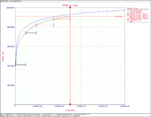
By clicking the Plot icon, we can then generate a plot that shows the nominal and actual idealized growth curve, the test termination time, the MTBF goal and the planned growth for each phase, as shown in Figure Growth Planning plot.

[math]\displaystyle{ }[/math]

Inputs for the Crow Extended model, when calculating the initial MTBF.

Inputs for the Crow Extended model when calculating the Growth Potential Design Margin.

Growth Planning window showing phase information, model inputs and results.

Growth planning plot.

Example 2

The reliability team of a product manufacturer is putting together a reliability growth plan for one of the new products under design. The reliability team wants to create an overall reliability growth plan based on the Crow Extended model. The inputs to the model are the following:

• The requirement or goal MTBF is [math]\displaystyle{ {{M}_{G}}=100 }[/math] hours.

• The Growth Potential Design Margin Factor is [math]\displaystyle{ GPDM=1.15 }[/math] .

• The Average Effectiveness Factor is [math]\displaystyle{ d\quad =0.6, }[/math] based on historical information for similar products developed by the company.

• The Management Strategy is [math]\displaystyle{ msr=0.90 }[/math] .

• The beta parameter for the discovery function, [math]\displaystyle{ h\left( t \right), }[/math] of the Type B failure modes is [math]\displaystyle{ \beta =0.71 }[/math] , based on data analysis of the previous product development project that was of similar nature.

• The test will be conducted in seven phases. The cumulative phase end times are [math]\displaystyle{ {{T}_{1}}=4000,{{T}_{2}}=8000 }[/math] , [math]\displaystyle{ {{T}_{3}}=12000, }[/math] [math]\displaystyle{ {{T}_{4}}=20000, }[/math]

• [math]\displaystyle{ {{T}_{5}}=25000, }[/math] [math]\displaystyle{ {{T}_{6}}=30000 }[/math] and [math]\displaystyle{ {{T}_{7}}=40000 }[/math] hours. The average fix delay for each phase is one week. For the first two phases, the plan is to test 1000 hours per week, so the average fix delay in terms of test hours for Phases 1 and 2 is [math]\displaystyle{ {{L}_{1}}=1000 }[/math] and hours. For Phases 3 and 4, the prototype test units are planned to be doubled, so the average fix delay in terms of test hours within one week also is going to be doubled, so we have: [math]\displaystyle{ {{L}_{3}}=2000 }[/math] and [math]\displaystyle{ {{L}_{4}}=2000 }[/math] hours. For Phases 5 and 6, a second shift is going to be added, so the amount of test hours within a week is going to be doubled again. Therefore, the average fix delay in terms of test hours within one week also is going to be doubled: [math]\displaystyle{ {{L}_{5}}=4000 }[/math] and [math]\displaystyle{ {{L}_{6}}=4000 }[/math] hours. For the last phase, more units and weekend shifts are planned to be added, so the total test hours within one week are going to be 6000 hours. In accordance, the average fix delay in terms of test hours will be [math]\displaystyle{ {{L}_{7}}=6000 }[/math] hours.

Construct a reliability growth plan with RGA 7 and make sure that the goal MTBF can be met within the total test hours allocated for growth testing. If not, make necessary changes in the phase durations in order to meet the goal.

Solution
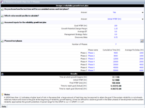
Figure 7 phases shows the planning input in RGA 7, in terms of test phases and average fix delays.

Figure Examplelanningalculations shows the planning calculations based on the goal MTBF of 100 hours and the rest of the known inputs into the model. As seen by the planning calculation results, the final actual MTBF at the end of the seventh phase is 98.66 hours, which is less than the MTBF goal of 100 hours. Also, in Figure results example 2, it is shown that the nominal time to meet the MTBF goal is 48420 hours, which is higher than the total test time that is currently planned to be allocated for reliability growth.

[math]\displaystyle{ }[/math]

Growth planning in seven phases.

Planning model inputs and results for the initial plan.

[math]\displaystyle{ }[/math]

Planning model with results for the initial plan.

Reliability growth plan with revised phase durations.

A new plan needs to be considered. The reliability team decides to increase the test time for Phases 5 and 6 to be 10000 hours each, instead of the 5000 hours that were considered in the initial plan. Also, the team decides to increase the duration of the seventh phase to 15000 hours. Since this is going to be achieved by testing for more calendar time in Phases 5, 6 and 7, the average fix delay during those phases is the same as the one in the initial plan. The test time per week is not going to be affected, only more weeks will be added to the schedule. Figure resived plan shows the revised plan, together with the calculated results. The actual time to meet the MTBF goal is now 54331 hours. The final MTBF that can be achieved at the end of the 55000 hours of growth testing is 100.04, which is slightly higher than the goal MTBF of 100 hours. The reliability team considers this plan as acceptable, since the MTBF goal will be met. Figure growth plot example 2 shows the overall reliability growth plan, with the nominal and actual growth curves, the MTBF goal line and the planned MTBF for each of the seven phases.

[math]\displaystyle{ }[/math]

Growth planning plot for the seven plhases with the revised plan.

Example 3

The reliability team of a product manufacturer has put together a reliability growth plan, based on the Crow Extended model, for one of their new products. The reliability growth model was constructed with the following inputs:

• The requirement or goal MTBF is [math]\displaystyle{ {{M}_{G}}=910 }[/math] hours.

• The Growth Potential Design Margin Factor is [math]\displaystyle{ GPDM=1.35 }[/math] .

• The Average Effectiveness Factor is [math]\displaystyle{ d\quad =0.7. }[/math]

• The Management Strategy is

• [math]\displaystyle{ msr=0.95 }[/math] .

• The beta parameter for the discovery function, [math]\displaystyle{ h\left( t \right), }[/math] of the Type B failure modes is [math]\displaystyle{ \beta =0.70 }[/math] .

• The test is planned to be conducted in four phases. The cumulative phase end times are [math]\displaystyle{ {{T}_{1}}=19000,{{T}_{2}}=38000 }[/math] , [math]\displaystyle{ {{T}_{3}}=70000 }[/math] and [math]\displaystyle{ {{T}_{4}}=100000 }[/math] . The average fix delay in terms of test hours for each phase is: [math]\displaystyle{ {{L}_{1}}=10000 }[/math] , [math]\displaystyle{ {{L}_{2}}=15000, }[/math] [math]\displaystyle{ {{L}_{3}}=20000 }[/math] and [math]\displaystyle{ {{L}_{4}}=25000 }[/math] hours.

1) Plot the nominal and actual reliability growth curves for this program, using RGA 7.

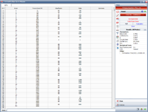
2) The reliability program was initiated and actual test data from Phase 1 is now available. The test data were analyzed using the Crow Extended - Continuous Evaluation model and Figure CECE data phase 1 shows the results. Note that the I events, which represent the times for implementation of fixes for BD modes, occur at least 10000 hours after the first occurrence of the specific BD mode. This is a reflection of the average fix delay being equal to 10000 hours for the first test phase. Of course we could have some exceptions that could have been fixed before 10000 hours after the first occurrence (i.e. discovery) of the mode, but on average, they should be fixed after 10000 hours.

The same applies to the delayed fixes at the end of Phase 1; on average there should be at least 10000 test hours between the discovery of the failure mode and the implementation of a fix for that mode, so failure modes discovered after 9000 hours of testing in the first phase cannot be implemented at the end of the first phase.

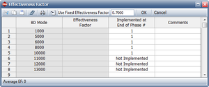
Figure EF window Example 3 shows the effectiveness factor window, where it is shown that fixes for failure modes BD 11000, BD 12000 and BD 13000 are not implemented at the end of the first phase due to the fix delay. The effectiveness factor used is in accordance with the planning model and has been fixed to 0.7.

[math]\displaystyle{ }[/math]

Phase 1 data, analyzed with the Crow Extended- Continuous Evaluation model.

Fixed effectiveness factor and phase of implementation for unfixed BD modes in Phase 1.

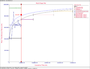
Construct a multi-phase graph that shows the analysis points for the test data in Phase 1, as compared to the nominal and actual idealized growth curves for this reliability growth plan. Is the program on track, so far, as compared to the plan?

Solution

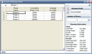
1) Figures inputs example 3 and planning info show the plan inputs, phase durations and average fix delays as entered in RGA 7, together with the results of the growth model. Figure plan plot shows the nominal and actual idealized growth curves for this program, together with the program MTBF goal.

[math]\displaystyle{ }[/math]

Inputs in reliability growth planning model.

[math]\displaystyle{ }[/math]

Reliability growth planning information and results.

Nominal and actual idealized growth curves with planned growth in four phases.

2) The next step is to associate the reliability growth plan with the data from phase 1. To do that, we right-click Additional Plots in the Project Explorer and choose Add MultiPhase Plot from the shortcut menu then follow the wizard to specify the data sheet that contains the phase 1 data with the Folio that defines the growth plan. Figure Multi-Phase shows the generated Multiple Phase Plot, which brings together the reliability growth planning model with the actual test results. This plot shows the demonstrated MTBF for each analysis point during the first phase of testing. Analysis points for projected and growth potential MTBF also can be plotted. For this example, it can be said that the program is on track since the demonstrated MTBF of the first phase is higher than the planned MTBF for that phase.

The Multiple Phase Plot can be continuously updated as the growth program progresses and more test data becomes available. In that manner, the reliability team can assess actual reliability performance against the established goals.

[math]\displaystyle{ }[/math]

Multi-Phase plot containing the overall growth plan and the actual test results for Phase 1.