Cumulative Damage Model for Progress Stress Profiles

ALTA_Reference_Examples_Banner.png

ALTA_Reference_Examples

Compares the results of a cumulative damage model for a ramp stress test.

Reference Case

The data set is from the table on page 232 in the book Accelerated Testing: Statistical Models, Test Plans, and Data Analysis by Dr. Nelson, John Wiley & Sons, 1990. The model of Eqn. (3.10) is used and the results are given in Section 3 of Table 3.2 on page 511.

Data

An accelerated test employed a pair of parallel disk electrodes immersed in insulating oil. The voltage V across the pair was increased linearly with time t at a specified rate, and then the voltage at oil breakdown was recorded. Since V = Rt (R is the ramp rate), the time to breakdown can be recorded. The breakdown time is also affected by the two electrode areas A. Three voltage linear rates and two electrode areas are used. The six stress profiles are:

Voltage Ramp Rate (Volts/sec)	Area (Sq. Inch)
10	1
100	1
1000	1
10	9
100	9
1000	9

The following table shows the failure data for an area of 1 square inch.

Time to Failure	Voltage Ramp Rate	Time to Failure	Voltage Ramp Rate	Time to Failure	Voltage Ramp Rate
41	10	46	100	55	1000
43	10	50	100	57	1000
42	10	39	100	59	1000
43	10	36	100	57	1000
44	10	47	100	55	1000
40	10	55	100	60	1000
38	10	49	100	53	1000
47	10	58	100	51	1000
43	10	50	100	57	1000
45	10	48	100	54	1000
38	10	53	100	57	1000
44	10	54	100	64	1000
49	10	55	100	53	1000
42	10	37	100	63	1000
42	10	53	100	51	1000
51	10	52	100	62	1000
39	10	53	100	62	1000
34	10	50	100	56	1000
41	10	52	100	62	1000
41	10	50	100	57	1000
35	10	45	100	41	1000
44	10	48	100	41	1000
46	10	53	100	51	1000
39	10	50	100	58	1000
41	10	43	100	59	1000
40	10	50	100	60	1000
52	10	42	100	58	1000
40	10	45	100	55	1000
35	10	47	100	59	1000
40	10	34	100	63	1000
39	10	46	100	63	1000
46	10	42	100	53	1000
47	10	46	100	63	1000
44	10	46	100	61	1000
41	10	52	100	59	1000
46	10	47	100	53	1000
46	10	53	100	60	1000
42	10	52	100	58	1000
45	10	45	100	62	1000
42	10	47	100	56	1000
44	10	43	100	69	1000
41	10	45	100	65	1000
44	10	54	100	51	1000
38	10	51	100	56	1000
36	10	46	100	55	1000
44	10	55	100	57	1000
50	10	44	100	54	1000
47	10	49	100	63	1000
49	10	49	100	65	1000
46	10	53	100	65	1000
34	10	53	100	56	1000
47	10	54	100	54	1000
49	10	53	100	65	1000
43	10	53	100	60	1000
43	10	51	100	60	1000
48	10	48	100	64	1000
34	10	49	100	60	1000
38	10	52	100	54	1000
47	10	45	100	57	1000
35	10	49	100	61	1000

The following table shows the failure data for an area of 9 square inch.

Time to Failure	Voltage Ramp Rate	Time to Failure	Voltage Ramp Rate	Time to Failure	Voltage Ramp Rate
33	10	43	100	50	1000
37	10	42	100	53	1000
38	10	45	100	50	1000
38	10	48	100	49	1000
38	10	38	100	53	1000
37	10	44	100	51	1000
27	10	37	100	47	1000
42	10	44	100	44	1000
39	10	43	100	53	1000
38	10	42	100	42	1000
42	10	43	100	49	1000
32	10	49	100	46	1000
42	10	44	100	50	1000
40	10	45	100	38	1000
32	10	50	100	48	1000
38	10	44	100	43	1000
36	10	44	100	52	1000
42	10	45	100	53	1000
20	10	41	100	52	1000
37	10	48	100	48	1000
43	10	45	100	45	1000
40	10	48	100	53	1000
38	10	43	100	52	1000
43	10	49	100	50	1000
39	10	50	100	55	1000
41	10	45	100	50	1000
35	10	45	100	43	1000
41	10	46	100	52	1000
40	10	47	100	50	1000
32	10	42	100	54	1000
38	10	47	100	51	1000
40	10	48	100	40	1000
37	10	47	100	52	1000
29	10	48	100	53	1000
31	10	39	100	47	1000
41	10	49	100	45	1000
38	10	44	100	53	1000
36	10	47	100	47	1000
35	10	34	100	54	1000
40	10	41	100	50	1000
37	10	45	100	32	1000
41	10	48	100	48	1000
36	10	44	100	53	1000
39	10	47	100	52	1000
43	10	45	100	45	1000
42	10	50	100	48	1000
43	10	40	100	48	1000
43	10	47	100	51	1000
41	10	47	100	53	1000
44	10	43	100	48	1000
37	10	49	100	54	1000
43	10	45	100	51	1000
38	10	45	100	50	1000
40	10	45	100	54	1000
40	10	47	100	35	1000
38	10	39	100	56	1000
33	10	44	100	51	1000
40	10	37	100	48	1000
35	10	47	100	48	1000
41	10	48	100	46	1000

Result

The following life stress relationship and Weibull distribution are used to analyze the data. At a constant stress V, the [math]\displaystyle{ \eta\,\! }[/math] is:

[math]\displaystyle{ ln\left(\eta(V, A)\right) = \alpha_{0}+\alpha_{1}ln(V)+\alpha_{2}ln(A)\,\! }[/math]

where V is the voltage and A is the area.

The reliability function at time t and stress V is:

[math]\displaystyle{ R(t,V,A) = e^{-\left(\frac{t}{\eta(V,A)} \right)^\beta}\,\! }[/math]

When stress is varying with time, the reliability at time t is given as follows:

[math]\displaystyle{ R(t,V,A) = e^{-\left(\int_{0}^{t}\frac{1}{\eta(x,A)}dx\right)^\beta} }[/math]

In the book, the following results are provided:

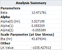
The ML solution for the parameters are given in Section 3 of Table 3.2 on page 511: [math]\displaystyle{ 1/\beta\,\! }[/math] = 0.07856677 ([math]\displaystyle{ \beta\,\! }[/math]=12.728027) , [math]\displaystyle{ \alpha_{0}\,\! }[/math] = 3.673202 , [math]\displaystyle{ \alpha_{1} = \,\! }[/math]0.05843506 , and [math]\displaystyle{ \alpha_{2}=\,\! }[/math]-0.058626.
The maximum log likelihood is -1035.4269.

Results in ALTA

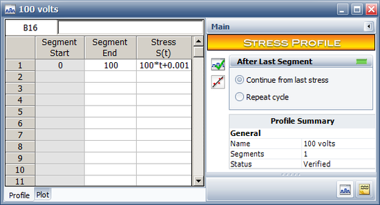
First, we create a stress profile in ALTA for each of three ramp rates: 10 volts/sec, 100 volts/sec and 1,000 volts/sec. For example, the following picture shows the stress profile for the 100 volts/sec ramp rate.

Note that the log transformation is used for voltage. At time 0, the voltage value will be 0 if the profile is defined as V(t) = 100*t; therefore, to define this stress profile, we add a small number (i.e., 0.001) to the voltage function.

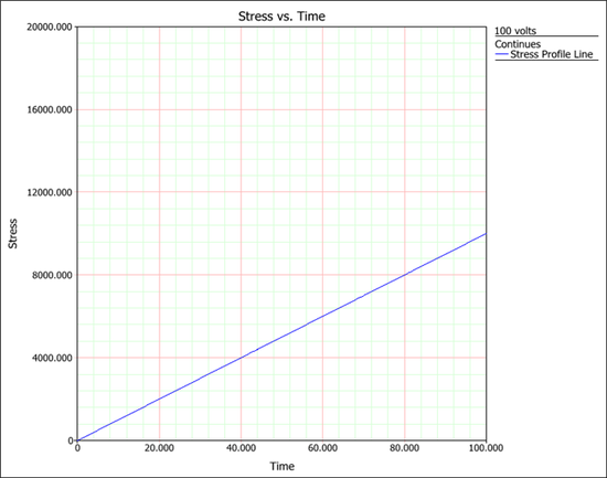
The following picture shows the plot for this stress profile.

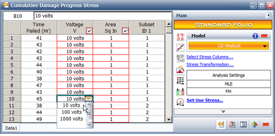
The next step is to enter the failure data into an ALTA standard folio and then use the stress profiles to define the stress values, as shown next.

The log transformation is used for both stresses. The results in ALTA show that the calculated parameters are close to the results in the book, while the log likelihood value (LK Value) is exactly the same as the value given in the book, as shown next.

Validate the Likelihood Value Calculation in ALTA

For the ML solution given in the book, the log likelihood value is -1035.4269.

Cumulative Damage Model for Progress Stress Profiles

Navigation menu

Search