Central Composite Response Surface Method: Difference between revisions

From ReliaWiki
Jump to navigation Jump to search
No edit summary
No edit summary
Line 15: Line 15:
!style="background:#f0f0f0;"|A
!style="background:#f0f0f0;"|B
!style="background:#f0f0f0;"|Y( yield)
!style="background:#f0f0f0;"|Y (yield)
|-
|-
| 8076.580||170||-1||-1||76.5
| 8076.580||170||-1||-1||76.5

Revision as of 16:10, 30 July 2015

DOE Reference Examples Banner.png


New format available! This reference is now available in a new format that offers faster page load, improved display for calculations and images and more targeted search.

As of January 2024, this Reliawiki page will not continue to be updated. Please update all links and bookmarks to the latest references at DOE examples and DOE reference examples.

Central Composite Response Surface Method

This example validates the calculation of the central composite response surface method in DOE++.

Reference Case

The data is from Example 11-1 on page 431 in the book Design and Analysis of Experiments by Douglas C. Montgomery, John Wiley & Sons, 2001.

Data

Natural Variables Coded Variables Responses
A (time) B (temperature) A B Y (yield)
8076.580 170 -1 -1 76.5
80 180 -1 1 77
90 170 1 -1 78
90 180 1 1 79.5
85 175 0 0 79.9
85 175 0 0 80.3
85 175 0 0 80.0
85 175 0 0 79.7
85 175 0 0 79.8
92.07 175 1.414 0 78.4
77.93 175 -1.414 0 75.6
85 182.07 0 1.414 78.5
85 167.93 0 -1.414 77

Result

From the book, the ANOVA table is:

Source Sum of Squares (Partial SS) DF Mean Square F value Prob > F
Model 28.25 5 5.65 79.85 <0.0001
A 7.92 1 7.92 111.93 <0.0001
B 2.12 1 2.12 30.01 0.0009
A∙A 13.18 1 13.18 186.22 <0.0001
B∙B 6.97 1 6.97 98.56 <0.0001
A∙B 0.25 1 0.25 3.53 0.1022
Residual 0.5 7 0.071
Lack of Fit 0.28 3 0.094 1.78 0.2897
Pure Error 0.21 4 0.053
Total 28.74 12

The final equation in terms of the actual values of these two factors is:


[math]\displaystyle{ \begin{align} Yield= -1430.52285+7.80749 * time + 13.27053 * temp-0.05505 * time^2 - 0.04005 * temp^2 + 0.01 * time * temp \end{align} }[/math]


The maximum yield is achieved at 80.21 with time=87 minutes and temperature=176.5 F.


Results in DOE++

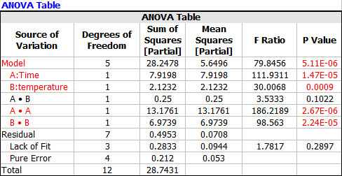
The software results match the book results. The ANOVA table is:

Composite anova.png

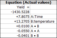
The final equation in terms of the actual factors is:

Composite final.png

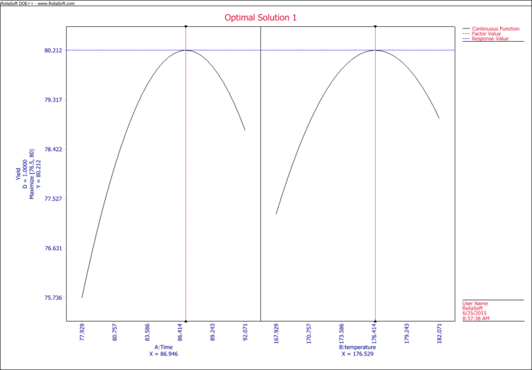
The maximum yield is achieved at 80.21, as shown in the optimization plot. The values at the red dash line are the optimal values for factor A and factor B. The blue line is corresponding to the maximum Y value.

Composite plot.png