Cumulative Damage Model for Progress Stress Profiles: Difference between revisions
Jump to navigation
Jump to search
Kate Racaza (talk | contribs) No edit summary |
Kate Racaza (talk | contribs) No edit summary |
||
| (3 intermediate revisions by the same user not shown) | |||
| Line 1: | Line 1: | ||
{{Reference Example|{{Banner ALTA Reference Examples}}}} | {{Reference Example|{{Banner ALTA Reference Examples}}}} | ||
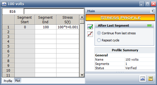
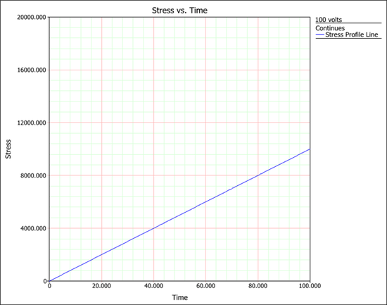
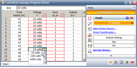
This example validates the results of a cumulative damage model for a ramp stress test in an ALTA standard folio. | |||
| Line 349: | Line 349: | ||
'''Validate the Likelihood Value Calculation in ALTA''' | '''Validate the Likelihood Value Calculation in ALTA''' | ||
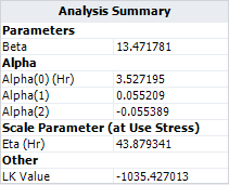
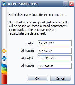
For the ML solution given in the book, the log likelihood value is -1035.4269. | For the ML solution given in the book, the log likelihood value is -1035.4269. To validate what the LK value would be if the parameter values used in the book were calculated in ALTA, we use the Alter Parameters tool, as shown next. | ||
[[Image: Cum Damage_Stress Profile_alter parameters.png|center]] | |||
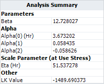
The resulting LK Value is -1489.6904, as shown next. | |||
[[Image: Cum Damage_Stress Profile_alter parameters results.png|center]] | |||
We need to validate the calculation for the log likelihood value in ALTA to make sure it is correct. | |||
First, we define the life characteristic of the Weibull distribution as a function of the two stresses: | |||
::<math>C = \int^{t}_{0} \frac{1}{\eta(V,A)} dV = \int^{t}_{0} e^{-(\alpha_{0}+\alpha_{1} \cdot ln(R \cdot V)+\alpha_{2} \cdot ln A)} dV\,\!</math> | |||
We get the equation for ''C'' as: | |||
::<math>C = e^{-\alpha_{0}} \cdot A^{-\alpha_{2}} \cdot R^{-\alpha_{1}} \cdot \frac{1}{1-\alpha_{1}} \cdot t^{1-\alpha_{1}}\,\!</math> | |||
where ''R'' is the ramping rate for the voltage. | |||
Therefore, the probability density function at failure time ''t'' is: | |||
::<math>f(t) = \beta \cdot e^{-C^{\beta}} \cdot C^{\beta} \cdot (1-\alpha_{1}) \cdot \frac{1}{t}\,\!</math> | |||
The following table shows the value for the pdf and its log transformation for the first several failure times. The log likelihood value for all other failure times can be calculated using the same method. The total log likelihood value is the sum of all the individual log likelihood values. | |||
{| {{table}} | |||
! Time to Failure||Voltage Ramp Rate||Area||f(t)||log-f(t) | |||
|- | |||
| 41||10||1||0.069249||-2.67004 | |||
|- | |||
| 43||10||1||0.094154||-2.36283 | |||
|- | |||
| 42||10||1||0.08244||-2.49568 | |||
|- | |||
| 43||10||1||0.094154||-2.36283 | |||
|- | |||
| 44||10||1||0.102165||-2.28117 | |||
|- | |||
| 40||10||1||0.05623||-2.8783 | |||
|- | |||
| 38||10||1||0.034243||-3.37427 | |||
|- | |||
| 47||10||1||0.083568||-2.4821 | |||
|- | |||
| 43||10||1||0.094154||-2.36283 | |||
|- | |||
| 45||10||1||0.104043||-2.26295 | |||
|- | |||
| …||…||…||…||… | |||
|- | |||
|colspan="4" style="text-align: right;"|'''Total'''||-1035.42696 | |||
|- | |||
|} | |||
The total likelihood value is LKV = -2.67004 -2.36283--2.49568…= -1035.42696. | |||
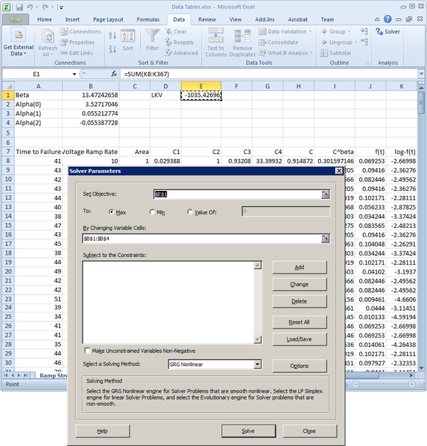
We also can use the optimization tool in Excel to find the ML solutions for this data set. By using the GRG-nonlinear optimization method provided by the "Solver Add-in" program in Excel, the result in Excel is the same as the result in ALTA. | |||
[[Image: Cum Damage_Stress Profile_excel add in.png|center|600 px]] | |||
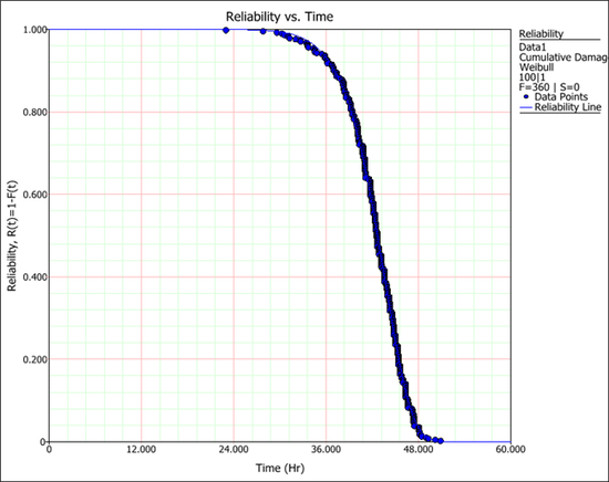
The following reliability plot shows that the predicted values (the line) from the model in ALTA can match the observed values (the points) very well. | |||
[[Image: Cum Damage Stress Profile plot.png|center|550 px]] | |||
Latest revision as of 18:23, 28 September 2015
New format available! This reference is now available in a new format that offers faster page load, improved display for calculations and images and more targeted search.
As of January 2024, this Reliawiki page will not continue to be updated. Please update all links and bookmarks to the latest references at ALTA examples and ALTA reference examples.

