New format available! This reference is now available in a new format that offers faster page load, improved display for calculations and images and more targeted search.
As of January 2024, this Reliawiki page will not continue to be updated. Please update all links and bookmarks to the latest references at RGA examples and RGA reference examples.
This example validates the results for test-find-test data in RGA.
Reference Case
International Standard IEC 61164 (Reliability Growth in Product Design and Test – Statistical Test and Estimation Methods), Example 4, pg. 32.
For this example, the following will be calculated:
- Parameters of the Crow Extended model
- Unseen BD mode failure intensity
- Cramér-von Mises (CVM) goodness of fit for BD modes
- Demonstrated MTBF (DMTBF)
- Projected PMTBF (PMTBF)
Data
The following table shows the data.
| Failure Time
|
Classification Mode
|
| 150 |
BD1
|
| 253 |
BD2
|
| 475 |
BD3
|
| 540 |
BD4
|
| 564 |
BD5
|
| 636 |
A
|
| 722 |
BD5
|
| 871 |
A
|
| 996 |
BD6
|
| 1003 |
BD7
|
| 1025 |
A
|
| 1120 |
BD8
|
| 1209 |
BD2
|
| 1255 |
BD9
|
| 1334 |
BD10
|
| 1647 |
BD9
|
| 1774 |
BD10
|
| 1927 |
BD11
|
| 2130 |
A
|
| 2214 |
A
|
| 2293 |
A
|
| 2448 |
A
|
| 2490 |
BD12
|
| 2508 |
A
|
| 2601 |
BD1
|
| 2635 |
BD8
|
| 2731 |
A
|
| 2747 |
BD6
|
| 2850 |
BD13
|
| 3040 |
BD9
|
| 3154 |
BD4
|
| 3171 |
A
|
| 3206 |
A
|
| 3245 |
DB12
|
| 3249 |
BD10
|
| 3420 |
BD5
|
| 3502 |
BD3
|
| 3646 |
BD10
|
| 3649 |
A
|
| 3663 |
BD2
|
| 3730 |
BD8
|
| 3794 |
BD14
|
| 3890 |
BD15
|
| 3949 |
A
|
| 3952 |
BD16
|
Termination Time = 4000 hours
| BD Mode
|
EF
|
| 1 |
0.7
|
| 2 |
0.7
|
| 3 |
0.8
|
| 4 |
0.8
|
| 5 |
0.9
|
| 6 |
0.9
|
| 7 |
0.5
|
| 8 |
0.8
|
| 9 |
0.9
|
| 10 |
0.7
|
| 11 |
0.7
|
| 12 |
0.6
|
| 13 |
0.6
|
| 14 |
0.7
|
| 15 |
0.7
|
| 16 |
0.5
|
Result
The book has the following results:
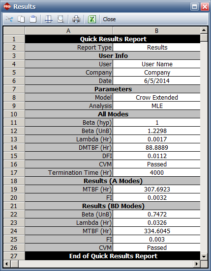
- BetaBD (UnB) = 0.7472, LambdaBD = 0.0326
- Unseen BD Mode Failure Intensity = 0.0030/hr
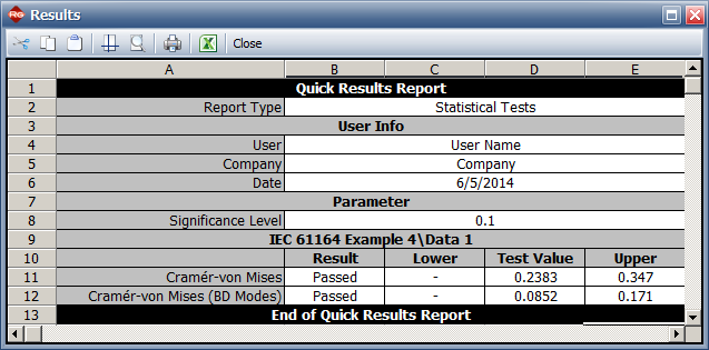
- Goodness of fit for BD modes: CVM = 0.085, critical value = 0.171 with significance level = 0.1. Since CVM < critical value can fail to reject hypothesis that the model fits the data.
Results in RGA
In RGA, the Crow Extended model with the maximum likelihood estimation (MLE) method was used to calculate the results.
For a test-find-test, the assumption is [math]\displaystyle{ \,\!\beta =1 }[/math]. Therefore:
- [math]\displaystyle{ \begin{align}
DMTBF=&\frac{T}{N}\\
\\
=&\frac{4000}{45}\\
\\
=&88.8889\; \; \mathrm{hours}
\end{align}\,\! }[/math]
- The model parameters are:
- [math]\displaystyle{ \begin{align}
\lambda _{p}=&\lambda _{A}+\sum_{i=1}^{N_{BD}}\left ( 1-d_{i} \right )\lambda _{i}+\bar{d}h\left ( T \right )\\
\\
=&\frac{N_{A}}{T}+\sum_{i=1}^{N_{BD}}\left ( 1-d_{i} \right )\frac{N_{i}}{T}+\bar{d}\lambda _{BD}\beta _{BD}T^{\beta -1}\\
\\
=&\frac{13}{4000}+0.002+\left ( 0.7188 \right )\left ( 0.032572 \right )\left ( 0.74715 \right )\left ( 4000 \right )^{0.7472-1}\\
\\
=&0.007398\\
\\
PMTBF=&\frac{1}{\lambda _{p}}\\
\\
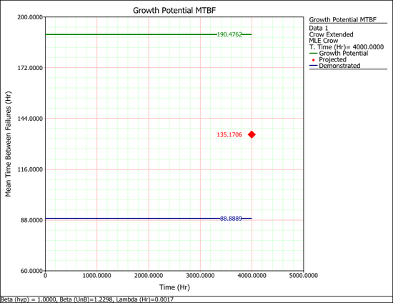
=&135.17 \; \; \mathrm{hours}
\end{align}\,\! }[/math]
- The growth potential MTBF plot:


