New format available! This reference is now available in a new format that offers faster page load, improved display for calculations and images and more targeted search.
As of January 2024, this Reliawiki page will not continue to be updated. Please update all links and bookmarks to the latest references at RGA examples and RGA reference examples.
|
Repairable Systems Analysis
|
This example validates the results for a repairable systems analysis in RGA.
Reference Case
Crow, L.H., Reliability Analysis for Complex Repairable Systems, Reliability and Biometry: Statistical Analysis of Lifelength, pg. 385, 1974.
For this example, the Power Law model parameters will be calculated.
Data
The following table shows the data.
| System 1
|
System 2
|
System 3
|
| 4.3 |
0.1 |
8.4
|
| 4.4 |
5.6 |
32.4
|
| 10.2 |
18.6 |
44.7
|
| 23.5 |
19.5 |
48.4
|
| 23.8 |
24.2 |
50.6
|
| 26.4 |
26.7 |
73.6
|
| 74 |
45.1 |
98.7
|
| 77.1 |
45.8 |
112.2
|
| 92.1 |
72.7 |
129.8
|
| 197.2 |
75.7 |
136
|
|
98.6 |
195.8
|
|
120.1 |
|
|
161.8 |
|
|
180.6 |
|
|
190.8 |
|
Simulated Data for 3 Systems with End Time = 200 hours
Result
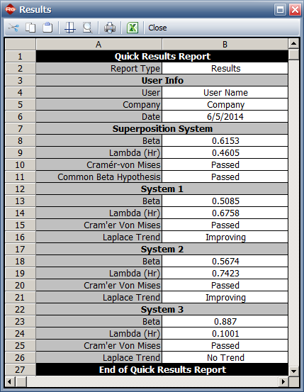
The book has the following results:
Beta = 0.615, Lambda = 0.461
Results in RGA
Since [math]\displaystyle{ \,\!S_{1}=S_{2}=S_{3}=0 }[/math] and [math]\displaystyle{ \,\!T_{1}=T_{2}=T_{3}=200 }[/math] then the maximum likelihood estimates of [math]\displaystyle{ \,\!\hat{\beta} }[/math] and [math]\displaystyle{ \,\!\hat{\lambda } }[/math] are given by:
- [math]\displaystyle{ \begin{align}
\hat{\beta} =&\frac{\underset{q=1}{\overset{K}{\mathop \sum }}N_{q}}{\underset{q=1}{\overset{K}{\mathop \sum }}\,\underset{i=1}{\overset{N_{q}}{\mathop \sum }}\ln \left ( \frac{T}{X_{iq}} \right )}\\
\\
=&0.6153
\end{align}\,\! }[/math]
- [math]\displaystyle{ \begin{align}
\hat{\lambda }=&\frac{{\underset{q=1}{\overset{K}{\mathop \sum }}N_{q}}}{KT^{\hat{\beta }}}\\
\\
=&0.4605
\end{align}\,\! }[/math]
The model parameters are:

