RGA Monte Carlo Simulation Example
New format available! This reference is now available in a new format that offers faster page load, improved display for calculations and images and more targeted search.
As of January 2024, this Reliawiki page will not continue to be updated. Please update all links and bookmarks to the latest references at RGA examples and RGA reference examples.
This example appears in the Reliability growth reference.
A reliability engineer wants to experiment with different testing scenarios as the reliability growth test of the company's new product is being prepared. From the reliability growth test data of a similar product that was developed previously, the beta and lambda parameters are [math]\displaystyle{ \beta =0.5\,\! }[/math] and [math]\displaystyle{ \lambda =0.75.\,\! }[/math] Three systems are to be used to generate a representative data set of expected times-to-failure for the upcoming test. The purpose is to explore different test durations in order to demonstrate an MTBF of 200 hours.
Solution
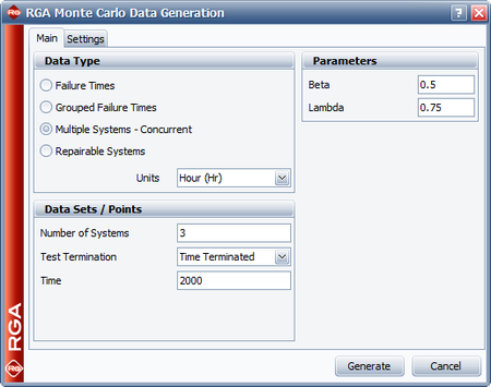
In the Monte Carlo window, the parameters are set to [math]\displaystyle{ \beta =0.5\,\! }[/math] and [math]\displaystyle{ \lambda =0.75.\,\! }[/math] Since we have three systems, we use the "multiple systems - concurrent" data sheet and then set the number of systems to 3. Initially, the test is set to be time terminated with 2,000 operating hours per system, for a total of 6,000 operating hours. The next figure shows the Monte Carlo window for this example.
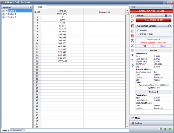
The next figure shows the generated failure times data. In this folio, the Advanced Systems View is used, so the data sheet shows the times-to-failure for system 2.
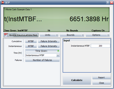
The data can then be analyzed just like a regular folio in the RGA software. In this case, we are interested in analyzing the data with the Crow-AMSAA (NHPP) model to calculate the demonstrated MTBF at the end of the test. In the Results area of the folio (shown in the figure above), it can be seen that the demonstrated MTBF at the end of the test is 189.83 hours. Since that does not meet the requirement of demonstrating an MTBF of 200 hours, we can either generate a new Monte Carlo data set with different time termination settings, or access the Quick Calculation Pad (QCP) in this folio to find the time for which the demonstrated (instantaneous) MTBF becomes 200 hours, as shown in the following figure. From the QCP it can be seen that, based on this specific data set, 6651.38 total operating hours are needed to show a demonstrated MTBF of 200 hours.
Note that since the Monte Carlo routine generates random input variables that follow the NHPP based on the specific [math]\displaystyle{ \beta \,\! }[/math] and [math]\displaystyle{ \lambda \,\! }[/math] values, if the same seed is not used the failure times will be different the next time you run the Monte Carlo routine. Also, because the input variables are pulled from an NHPP with the expected values of [math]\displaystyle{ \beta \,\! }[/math] and [math]\displaystyle{ \lambda ,\,\! }[/math] it should not be expected that the calculated parameters of the generated data set will match exactly the input parameters that were specified. In this example, the input parameters were set as [math]\displaystyle{ \beta =0.5\,\! }[/math] and [math]\displaystyle{ \lambda =0.75\,\! }[/math], and the data set based on the Monte Carlo generated failure times yielded Crow-AMSAA (NHPP) parameters of [math]\displaystyle{ \beta =0.4939\,\! }[/math] and [math]\displaystyle{ \lambda =0.8716\,\! }[/math]. The next time a data set is generated with a random seed, the calculated parameters will be slightly different, since we are essentially pulling input variables from a predefined distribution. The more simulations that are run, the more the calculated parameters will converge with the expected parameters. In the RGA software, the total number of generated failures with the Monte Carlo utility has to be less than 64,000.


