Optimal Custom Designs
Although two level fractional factorial designs, Plackett-Burman designs, Taguchi orthogonal array and other predefined designs are enough for most applications, sometimes these designs may not be sufficient due to constraints on available resources such as time, cost and factor values. Therefore, in this chapter, we will discuss how to create an optimal custom design. A DOE folio has two types of optimal custom designs: regression model-based and distance-based.
Regression Model-Based Optimal Designs
Regression model-based optimal designs are optimal for a selected regression model. Therefore, a regression model must first be specified. The regression model should include all the effects that the experimenters are interested in.
As discussed in the linear regression chapter, the following linear equation is used in DOE data analysis.
- [math]\displaystyle{ y={{\beta }_{0}}+{{\beta }_{1}}{{x}_{1}}+\cdot \cdot \cdot +{{\beta }_{p}}{{x}_{p}}+\varepsilon \,\! }[/math]
where:
• [math]\displaystyle{ y\,\! }[/math] is the response
• [math]\displaystyle{ {{x}_{1}}\,\! }[/math], …, [math]\displaystyle{ {{x}_{p}}\,\! }[/math] are the factors
• [math]\displaystyle{ {{\beta }_{0}}\,\! }[/math], [math]\displaystyle{ {{\beta }_{1}}\,\! }[/math], …,
• [math]\displaystyle{ {{\beta }_{p}}\,\! }[/math] are model coefficients
• [math]\displaystyle{ \varepsilon \,\! }[/math] is the error term
For each run, the above equation becomes:
- [math]\displaystyle{ {{y}_{i}}={{\beta }_{0}}+{{\beta }_{1}}{{x}_{i1}}+\cdot \cdot \cdot {{\beta }_{p}}{{x}_{ip}}+{{\varepsilon }_{i}}\,\! }[/math]
It can be written in matrix notation as:
- [math]\displaystyle{ Y=X\beta +\varepsilon \,\! }[/math]
where:
- [math]\displaystyle{ Y=\left[ \begin{matrix} {{y}_{1}} \\ \vdots \\ {{y}_{n}} \\ \end{matrix} \right]\,\! }[/math]
, [math]\displaystyle{ X=\left[ \begin{matrix} 1 & {{x}_{11}} & \cdots & {{x}_{1p}} \\ \vdots & \vdots & \ddots & \vdots \\ 1 & {{x}_{n1}} & \cdots & {{x}_{np}} \\ \end{matrix} \right]\,\! }[/math] , [math]\displaystyle{ \beta =\left[ \begin{matrix} {{\beta }_{1}} \\ \vdots \\ {{\beta }_{n}} \\ \end{matrix} \right]\,\! }[/math] , [math]\displaystyle{ \varepsilon =\left[ \begin{matrix} {{\varepsilon }_{1}} \\ \vdots \\ {{\varepsilon }_{n}} \\ \end{matrix} \right]\,\! }[/math]
n is the total number of samples or runs. As discussed in the design evaluation chapter, the information matrix for an experiment is:
- [math]\displaystyle{ I=X'X\,\! }[/math]
The variance and covariance matrix for the regression coefficients is:
- [math]\displaystyle{ \Sigma ={{\sigma }^{2}}{{\left( X'X \right)}^{-1}}\,\! }[/math]
where [math]\displaystyle{ {{\sigma }^{2}}\,\! }[/math] is the variance of the error [math]\displaystyle{ \varepsilon \,\! }[/math]. It can be either specified by experimenters from their engineering knowledge or estimated from the data analysis. If the number of available samples is given, we need to choose the value of [math]\displaystyle{ {{x}_{ij}}\,\! }[/math] in matrix [math]\displaystyle{ X\,\! }[/math] to minimize the determinant of [math]\displaystyle{ \Sigma \,\! }[/math]. A small determinate means less uncertainty of the estimated coefficients [math]\displaystyle{ \beta \,\! }[/math]. This is the same as maximizing the determinant of [math]\displaystyle{ X'X\,\! }[/math]. A design that uses the determinant as the objective is called D-optimal design. A D-optimal design can be either selected from a standard design or created based on the values of factors without creating a standard design first. In this chapter, we discuss how to select a D-optimal design from a standard factorial design.
Select a D-Optimal Custom Design from a Standard Design
Assume that we need to design an experiment to investigate five factors with two levels each. To run a full factorial design, a total of [math]\displaystyle{ {{2}^{5}}=32\,\! }[/math] factor combinations are needed. However, only 11 samples are available. To obtain the most information, which of the 11 factor combinations from the total of 32 should be applied to these 11 samples? To answer this question, we need to first decide what information we want to obtain.
The 32 runs required for a full factorial design are given in the table below.
Order A B C D E 1 -1 -1 -1 -1 -1 2 1 -1 -1 -1 -1 3 -1 1 -1 -1 -1 4 1 1 -1 -1 -1 5 -1 -1 1 -1 -1 6 1 -1 1 -1 -1 7 -1 1 1 -1 -1 8 1 1 1 -1 -1 9 -1 -1 -1 1 -1 10 1 -1 -1 1 -1 11 -1 1 -1 1 -1 12 1 1 -1 1 -1 13 -1 -1 1 1 -1 14 1 -1 1 1 -1 15 -1 1 1 1 -1 16 1 1 1 1 -1 17 -1 -1 -1 -1 1 18 1 -1 -1 -1 1 19 -1 1 -1 -1 1 20 1 1 -1 -1 1 21 -1 -1 1 -1 1 22 1 -1 1 -1 1 23 -1 1 1 -1 1 24 1 1 1 -1 1 25 -1 -1 -1 1 1 26 1 -1 -1 1 1 27 -1 1 -1 1 1 28 1 1 -1 1 1 29 -1 -1 1 1 1 30 1 -1 1 1 1 31 -1 1 1 1 1 32 1 1 1 1 1
Since only 11 test samples are available, we must choose 11 factor value combinations from the above table. The experiment also has the following constraints:
• Due to safety concerns, it is not allowed to set all the factors at their high level at the same time. Therefore, we cannot use run number 32 in the experiment.
• The engineers are very interested in checking the response at A=D=1, and B=C=E=-1. Therefore, run number 10 must be included in the experiment.
• The engineers need to check the main effects and the interaction effect of AE. Therefore, the model for designing the optimal customer design is:
- [math]\displaystyle{ y={{\beta }_{0}}+{{\beta }_{1}}A+{{\beta }_{2}}B+{{\beta }_{3}}C+{{\beta }_{4}}D+{{\beta }_{5}}E+{{\beta }_{15}}AE+\varepsilon \,\! }[/math]
Since run number 10 must be included, there are only 10 runs left to choose from the above table. Many algorithms can be used to choose these 10 runs to maximize the determinant of the information matrix.
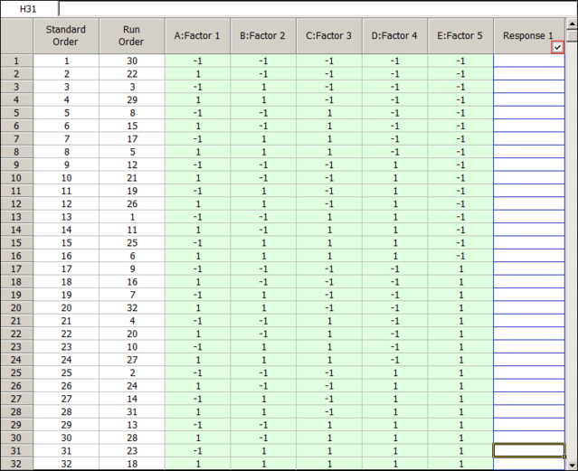
For this example, we first need to create a regular two level factorial design with five factors, as shown next.
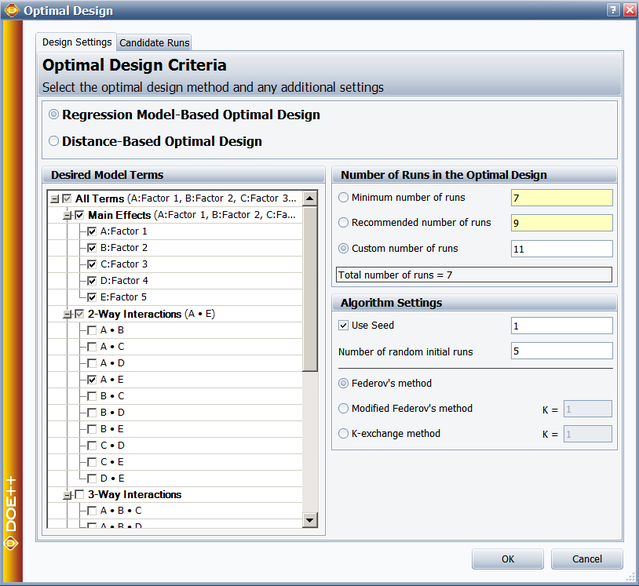
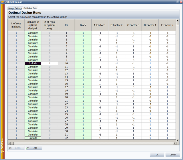
On the Design Settings tab of the Optimal Design window, you can select which terms to include in the model and specify the number of runs to be used in the experiment. Only main effects and AE are selected. The number of runs is set to 11. In the Candidate Runs tab of the window, run number 10 was set to be included and run number 32 was set to be excluded.
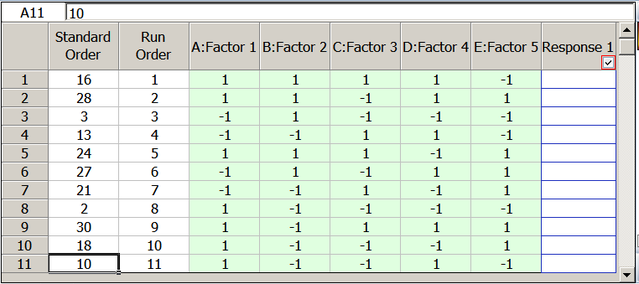
The resulting optimal custom design is shown next.
The design evaluation results for this design are given below.
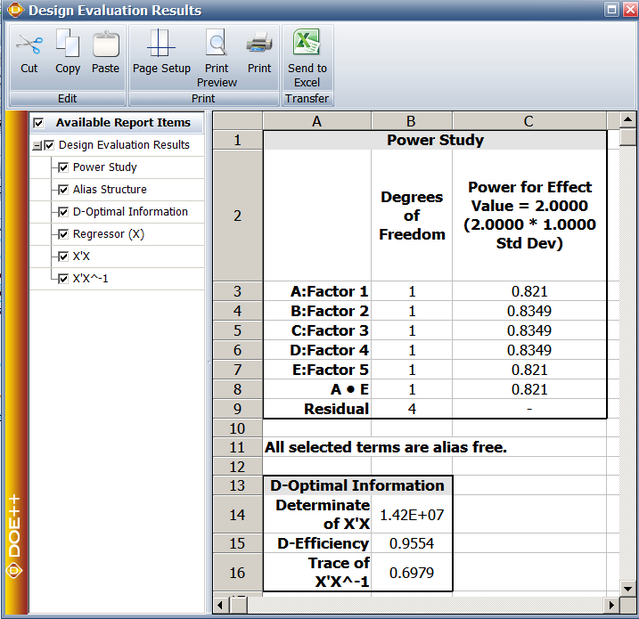
From the design evaluation results, we can see the generated design can clearly estimate all the main effects and the AE interaction. The determinate of the information matrix X’X is 1.42E+7 and the D-efficiency is 0.9554. The power for an effect of 2-standard deviation for each of the terms of interest is also given in the design evaluation.
Algorithms for Selecting Model-Based D-Optimal Designs
In a DOE folio, the Federov’s method, the modified Federov’s method and the k-exchange method are used to select test runs from all the candidates. They are briefly explained below.
The Federov algorithm [Fedorov, 1972]
Assume there is an initial optimal design with number of runs of n. The initial optimal design can be obtained using the sequential optimization method given in [Dykstra 1971, Galil and Kiefer 1980]. We need to exchange one of the rows in the initial design with one of the rows from the candidate runs. Let’s call the initial design [math]\displaystyle{ {{X}_{old}}\,\! }[/math] and call the design after row exchange [math]\displaystyle{ {{X}_{new}}\,\! }[/math]. The determinant of the new information matrix is:
- [math]\displaystyle{ \left| X_{new}^{'}{{X}_{new}} \right|=\left| X_{old}^{'}{{X}_{old}} \right|\times \left( 1+\Delta \left( {{x}_{i}},{{x}_{j}} \right) \right)\,\! }[/math]
where [math]\displaystyle{ {{x}_{i}}\,\! }[/math] is the row from the current optimal design. It needs to be exchanged with [math]\displaystyle{ {{x}_{j}}\,\! }[/math], a candidate run from the candidate set. [math]\displaystyle{ \Delta \left( {{x}_{j}},{{x}_{j}} \right)\,\! }[/math] is the amount of change in the determinant of the information matrix. It is calculated by:
- [math]\displaystyle{ \Delta \left( {{x}_{i}},{{x}_{j}} \right)=d\left( {{x}_{j}} \right)-\left[ d\left( {{x}_{i}} \right)d\left( {{x}_{j}} \right)-d{{({{x}_{i}},{{x}_{j}})}^{2}} \right]-d\left( {{x}_{i}} \right)\,\! }[/math]
where:
• [math]\displaystyle{ d({{x}_{i}},{{x}_{j}})=x_{i}^{'}{{\left( X_{old}^{'}{{X}_{old}} \right)}^{-1}}{{x}_{j}}\,\! }[/math] is the covariance for [math]\displaystyle{ {{x}_{i}}\,\! }[/math] and [math]\displaystyle{ {{x}_{j}}\,\! }[/math]
• [math]\displaystyle{ d\left( {{x}_{i}} \right)\,\! }[/math] and [math]\displaystyle{ d({{x}_{j}})\,\! }[/math] are the variance of [math]\displaystyle{ {{x}_{i}}\,\! }[/math] and [math]\displaystyle{ {{x}_{j}}\,\! }[/math]calculated using the current optimal design [math]\displaystyle{ {{X}_{old}}\,\! }[/math]
The basic idea behind the Fedorov algorithm is to calculate the delta-value for all the possible exchange pairs from the current design and the candidate runs, and then select the pair with the highest value. At each iteration, it calculates [math]\displaystyle{ n\times N\,\! }[/math] deltas (where n is the number of runs in the current design matrix and N is the number of runs in the candidate run matrix) and chooses the best one for exchange. The algorithm stops when the change of the determinate is less than a pre-defined small value.
The Modified Federov Algorithm [Cook and Nachtsheim, 1980]
The above Federov algorithm is very slow since it only conducts one exchange after calculating [math]\displaystyle{ n\times N\,\! }[/math]deltas. The modified Federov algorithm tries to improve the speed. It is a simplified version of the Fedorov method. Assume the current design matrix is [math]\displaystyle{ {{X}_{old}}\,\! }[/math]. The algorithm starts from the 1st row in the design matrix and uses it to calculate [math]\displaystyle{ 1\times N\,\! }[/math] deltas (deltas of this design run with all the candidate runs). An exchange is conducted if the largest delta is a positive value. The above steps are repeated until the increase of the determinant is less than a pre-defined small value. Therefore, the modified Federov algorithm results in one exchange after calculating N deltas.
The K-Exchange Algorithm [Johnson and Nachtsheim, 1983]
This is a variation of the modified Fedorov algorithm. Instead of calculating the deltas for all the design runs in one iteration, it calculates only the deltas for the k-worst runs. First, the algorithm uses the current design matrix to calculate the variance of each run in the design matrix. The k runs with the lowest variances are the runs that need to exchange. Then for each of the k worst runs, it calculates N deltas with all the N candidate runs. If the largest delta is greater than a pre-defined small value, then this row is exchanged with the candidate row, resulting in the largest positive delta. Once all the k points are exchanged, a new design matrix is obtained and the above steps are repeated until no exchange can be conducted. Usually k is set to be:[math]\displaystyle{ k\le n/4\,\! }[/math]where n is the number of runs in the optimal design. 2 Distance-Based Optimal Designs
Sometimes, experimenters want the design points (runs) in an experiment to cover as large of a design space as possible. In other words, the distance between design points is intended to be as far as possible. Distance-based optimal designs are used for this purpose.
To create a distance-based optimal design, the candidate runs should be available. First, the average value of each factor is calculated. This average is called the “center” of the design space. For qualitative factors, the average is calculated for the indicator variables in the regression model. For quantitative factors, the average is calculated based on the coded values. The distance of each candidate run to the center is calculated and sorted. The run with the largest distance is selected to be in the optimal design. If there are multiple runs with the same largest distance, a run is randomly selected from them. The “center” of the runs in the current optimal design is then calculated. The distances of all the available runs to this “center” are also calculated. Based on these distances, the next run is selected and put in the optimal design. Repeat this process until the required number of runs in the optimal design is reached.
Example: Three factors were investigated in an experiment. Factor A is Temperature and has two levels: 50C and 90C. Factor B is Time and it has three levels: 10, 20, and 30 minutes. Factor C is Humidity with four levels: 40%, 45%, 50%, and 55%. All three factors are quantitative. A complete factorial design would require 24 runs. The experimenters can only run 12 of them due to limitations on time and cost. The complete general full factorial design is given below.
The generated distance-based design with 12 runs is:
From the above generated design, we can see that for each factor, only its lowest and highest values are selected. By doing this, the distances between all the runs are maximized. Distance-based custom design can sometimes generate a design with aliased main effects. Maximizing the distance does not guarantee that the design can estimate all the main effects clearly. For this reason, using the D-optimal criterion is always preferred.
Reference for the Algorithms:
• Fedorov, V. V. (1972), “Theory of Optimal Experiments (Review)”, Biometrika, cvol. 59, no. 3, 697-698. Translated and edited by W. J. Studden and E. M. Klimko.
• Dykstra, O. (1971), “The augmentation of experimental data to maximize |X’X|, Technometrics, vol. 13, no. 3, 682-688.
• Galil, Z. and Kiefer, J. (1980), “Time and Space Saving Computer Methods, Related to Mitchell’s DETMAX, for Finding D-Optimal Designs”, Technometrics, vol. 22, no. 3, 301-313.
• Cook, R. D. and Nachtsheim, C. J. (1980), “A Comparison of Algorithms for Constructing Exact D-Optimal Designs,” Technometrics, vol. 22, no. 3, 315-324.
• Johnson, M. E. and Nachtsheim, C. J. (1983), “Some Guidelines for Constructing Exact D-Optimal Designs on Convex Design Spaces,” Technometrics , vol. 25, no. 3, 271-277.
