Lognormal Confidence Bounds

Confidence Bounds

The method used by the application in estimating the different types of confidence bounds for lognormally distributed data is presented in this section. Note that there are closed-form solutions for both the normal and lognormal reliability that can be obtained without the use of the Fisher information matrix. However, these closed-form solutions only apply to complete data. To achieve consistent application across all possible data types, Weibull++ always uses the Fisher matrix in computing confidence intervals. The complete derivations were presented in detail for a general function in Confidence Bounds. For a discussion on exact confidence bounds for the normal and lognormal, see The Normal Distribution.

Fisher Matrix Bounds

Bounds on the Parameters

The lower and upper bounds on the mean, [math]\displaystyle{ {\mu }'\,\! }[/math], are estimated from:

[math]\displaystyle{ \begin{align} & \mu _{U}^{\prime }= & {{\widehat{\mu }}^{\prime }}+{{K}_{\alpha }}\sqrt{Var({{\widehat{\mu }}^{\prime }})}\text{ (upper bound),} \\ & \mu _{L}^{\prime }= & {{\widehat{\mu }}^{\prime }}-{{K}_{\alpha }}\sqrt{Var({{\widehat{\mu }}^{\prime }})}\text{ (lower bound)}\text{.} \end{align}\,\! }[/math]

For the standard deviation, [math]\displaystyle{ {\widehat{\sigma}'}\,\! }[/math], [math]\displaystyle{ \ln ({{\widehat{\sigma'}}})\,\! }[/math] is treated as normally distributed, and the bounds are estimated from:

[math]\displaystyle{ \begin{align} & {{\sigma}_{U}}= & {{\widehat{\sigma'}}}\cdot {{e}^{\tfrac{{{K}_{\alpha }}\sqrt{Var({{\widehat{\sigma'}}})}}{{{\widehat{\sigma'}}}}}}\text{ (upper bound),} \\ & {{\sigma }_{L}}= & \frac{{{\widehat{\sigma'}}}}{{{e}^{\tfrac{{{K}_{\alpha }}\sqrt{Var({{\widehat{\sigma' }}})}}{{{\widehat{\sigma'}}}}}}}\text{ (lower bound),} \end{align}\,\! }[/math]

where [math]\displaystyle{ {{K}_{\alpha }}\,\! }[/math] is defined by:

[math]\displaystyle{ \alpha =\frac{1}{\sqrt{2\pi }}\int_{{{K}_{\alpha }}}^{\infty }{{e}^{-\tfrac{{{t}^{2}}}{2}}}dt=1-\Phi ({{K}_{\alpha }})\,\! }[/math]

If [math]\displaystyle{ \delta \,\! }[/math] is the confidence level, then [math]\displaystyle{ \alpha =\tfrac{1-\delta }{2}\,\! }[/math] for the two-sided bounds and [math]\displaystyle{ \alpha =1-\delta \,\! }[/math] for the one-sided bounds.

The variances and covariances of [math]\displaystyle{ {{\widehat{\mu }}^{\prime }}\,\! }[/math] and [math]\displaystyle{ {{\widehat{\sigma'}}}\,\! }[/math] are estimated as follows:

[math]\displaystyle{ \left( \begin{matrix} \widehat{Var}\left( {{\widehat{\mu }}^{\prime }} \right) & \widehat{Cov}\left( {{\widehat{\mu }}^{\prime }},{{\widehat{\sigma'}}} \right) \\ \widehat{Cov}\left( {{\widehat{\mu }}^{\prime }},{{\widehat{\sigma'}}} \right) & \widehat{Var}\left( {{\widehat{\sigma'}}} \right) \\ \end{matrix} \right)=\left( \begin{matrix} -\tfrac{{{\partial }^{2}}\Lambda }{\partial {{({\mu }')}^{2}}} & -\tfrac{{{\partial }^{2}}\Lambda }{\partial {\mu }'\partial {{\sigma'}}} \\ {} & {} \\ -\tfrac{{{\partial }^{2}}\Lambda }{\partial {\mu }'\partial {{\sigma'}}} & -\tfrac{{{\partial }^{2}}\Lambda }{\partial \sigma'^{2}} \\ \end{matrix} \right)_{{\mu }'={{\widehat{\mu }}^{\prime }},{{\sigma'}}={{\widehat{\sigma'}}}}^{-1}\,\! }[/math]

where [math]\displaystyle{ \Lambda \,\! }[/math] is the log-likelihood function of the lognormal distribution.

Bounds on Time (Type 1)

The bounds around time for a given lognormal percentile, or unreliability, are estimated by first solving the reliability equation with respect to time, as follows:

[math]\displaystyle{ {t}'({{\widehat{\mu }}^{\prime }},{{\widehat{\sigma' }}})={{\widehat{\mu }}^{\prime }}+z\cdot {{\widehat{\sigma' }}}\,\! }[/math]

where:

[math]\displaystyle{ z={{\Phi }^{-1}}\left[ F({t}') \right]\,\! }[/math]

and:

[math]\displaystyle{ \Phi (z)=\frac{1}{\sqrt{2\pi }}\int_{-\infty }^{z({t}')}{{e}^{-\tfrac{1}{2}{{z}^{2}}}}dz\,\! }[/math]

The next step is to calculate the variance of [math]\displaystyle{ {T}'({{\widehat{\mu }}^{\prime }},{{\widehat{\sigma }}}):\,\! }[/math]

[math]\displaystyle{ \begin{align} & Var({{{\hat{t}}}^{\prime }})= & {{\left( \frac{\partial {t}'}{\partial {\mu }'} \right)}^{2}}Var({{\widehat{\mu }}^{\prime }})+{{\left( \frac{\partial {t}'}{\partial {{\sigma' }}} \right)}^{2}}Var({{\widehat{\sigma' }}}) \\ & & +2\left( \frac{\partial {t}'}{\partial {\mu }'} \right)\left( \frac{\partial {t}'}{\partial {{\sigma' }}} \right)Cov\left( {{\widehat{\mu }}^{\prime }},{{\widehat{\sigma' }}} \right) \\ & & \\ & Var({{{\hat{t}}}^{\prime }})= & Var({{\widehat{\mu }}^{\prime }})+{{\widehat{z}}^{2}}Var({{\widehat{\sigma' }}})+2\cdot \widehat{z}\cdot Cov\left( {{\widehat{\mu }}^{\prime }},{{\widehat{\sigma' }}} \right) \end{align}\,\! }[/math]

The upper and lower bounds are then found by:

[math]\displaystyle{ \begin{align} & t_{U}^{\prime }= & \ln {{t}_{U}}={{{\hat{t}}}^{\prime }}+{{K}_{\alpha }}\sqrt{Var({{{\hat{t}}}^{\prime }})} \\ & t_{L}^{\prime }= & \ln {{t}_{L}}={{{\hat{t}}}^{\prime }}-{{K}_{\alpha }}\sqrt{Var({{{\hat{t}}}^{\prime }})} \end{align}\,\! }[/math]

Solving for [math]\displaystyle{ {{t}_{U}}\,\! }[/math] and [math]\displaystyle{ {{t}_{L}}\,\! }[/math] we get:

[math]\displaystyle{ \begin{align} & {{t}_{U}}= & {{e}^{t_{U}^{\prime }}}\text{ (upper bound),} \\ & {{t}_{L}}= & {{e}^{t_{L}^{\prime }}}\text{ (lower bound)}\text{.} \end{align}\,\! }[/math]

Bounds on Reliability (Type 2)

The reliability of the lognormal distribution is:

[math]\displaystyle{ \hat{R}(t;{{\hat{\mu }}^{'}},{{\hat{\sigma }}^{'}})=\int_{t'}^{\infty }{\frac{1}{{{{\hat{\sigma }}}^{'}}\sqrt{2\pi }}}{{e}^{-\frac{1}{2}{{\left( \frac{x-{{{\hat{\mu }}}^{'}}}{{{{\hat{\sigma }}}^{'}}} \right)}^{2}}}}dx\,\! }[/math]

where [math]\displaystyle{ t'=\ln (t)\,\! }[/math]. Let [math]\displaystyle{ \hat{z}(x)=\frac{x-{{{\hat{\mu }}}^{'}}}{{{\sigma }^{'}}}\,\! }[/math], the above equation then becomes:

[math]\displaystyle{ \hat{R}\left( \hat{z}(t') \right)=\int_{\hat{z}(t')}^{\infty }{\frac{1}{\sqrt{2\pi }}}{{e}^{-\frac{1}{2}{{z}^{2}}}}dz\,\! }[/math]

The bounds on [math]\displaystyle{ z\,\! }[/math] are estimated from:

[math]\displaystyle{ \begin{align} & {{z}_{U}}= & \widehat{z}+{{K}_{\alpha }}\sqrt{Var(\widehat{z})} \\ & {{z}_{L}}= & \widehat{z}-{{K}_{\alpha }}\sqrt{Var(\widehat{z})} \end{align}\,\! }[/math]

where:

[math]\displaystyle{ \begin{align} & Var(\hat{z})=\left( \frac{\partial {z}}{\partial \mu '} \right)_{\hat{\mu }'}^{2}Var\left( \hat{\mu }' \right)+\left( \frac{\partial {z}}{\partial \sigma '} \right)_{\hat{\sigma }'}^{2}Var\left( \hat{\sigma }' \right) \\ & +2\left( \frac{\partial{z}}{\partial \mu '} \right)_{\hat{\mu }'}^{{}}\left( \frac{\partial {z}}{\partial \sigma '} \right)_{\hat{\sigma }'}^{{}}Cov\left( \hat{\mu }',\hat{\sigma }' \right) \end{align}\,\! }[/math]

or:

[math]\displaystyle{ Var(\hat{z})=\frac{1}{{{{\hat{\sigma }}}^{'2}}}\left[ Var\left( \hat{\mu }' \right)+{{{\hat{z}}}^{2}}Var\left( \sigma ' \right)+2\cdot \hat{z}\cdot Cov\left( \hat{\mu }',\hat{\sigma }' \right) \right]\,\! }[/math]

The upper and lower bounds on reliability are:

[math]\displaystyle{ \begin{align} & {{R}_{U}}= & \int_{{{z}_{L}}}^{\infty }\frac{1}{\sqrt{2\pi }}{{e}^{-\tfrac{1}{2}{{z}^{2}}}}dz\text{ (Upper bound)} \\ & {{R}_{L}}= & \int_{{{z}_{U}}}^{\infty }\frac{1}{\sqrt{2\pi }}{{e}^{-\tfrac{1}{2}{{z}^{2}}}}dz\text{ (Lower bound)} \end{align}\,\! }[/math]

Likelihood Ratio Confidence Bounds

Bounds on Parameters

As covered in Parameter Estimation, the likelihood confidence bounds are calculated by finding values for [math]\displaystyle{ {{\theta }_{1}}\,\! }[/math] and [math]\displaystyle{ {{\theta }_{2}}\,\! }[/math] that satisfy:

[math]\displaystyle{ -2\cdot \text{ln}\left( \frac{L({{\theta }_{1}},{{\theta }_{2}})}{L({{\widehat{\theta }}_{1}},{{\widehat{\theta }}_{2}})} \right)=\chi _{\alpha ;1}^{2}\,\! }[/math]

This equation can be rewritten as:

[math]\displaystyle{ L({{\theta }_{1}},{{\theta }_{2}})=L({{\widehat{\theta }}_{1}},{{\widehat{\theta }}_{2}})\cdot {{e}^{\tfrac{-\chi _{\alpha ;1}^{2}}{2}}}\,\! }[/math]

For complete data, the likelihood formula for the normal distribution is given by:

[math]\displaystyle{ L({\mu }',{{\sigma' }})=\underset{i=1}{\overset{N}{\mathop \prod }}\,f({{x}_{i}};{\mu }',{{\sigma' }})=\underset{i=1}{\overset{N}{\mathop \prod }}\,\frac{1}{{{x}_{i}}\cdot {{\sigma' }}\cdot \sqrt{2\pi }}\cdot {{e}^{-\tfrac{1}{2}{{\left( \tfrac{\text{ln}({{x}_{i}})-{\mu }'}{{{\sigma'}}} \right)}^{2}}}}\,\! }[/math]

where the [math]\displaystyle{ {{x}_{i}}\,\! }[/math] values represent the original time-to-failure data. For a given value of [math]\displaystyle{ \alpha \,\! }[/math], values for [math]\displaystyle{ {\mu }'\,\! }[/math] and [math]\displaystyle{ {{\sigma' }}\,\! }[/math] can be found which represent the maximum and minimum values that satisfy likelihood ratio equation. These represent the confidence bounds for the parameters at a confidence level [math]\displaystyle{ \delta ,\,\! }[/math] where [math]\displaystyle{ \alpha =\delta \,\! }[/math] for two-sided bounds and [math]\displaystyle{ \alpha =2\delta -1\,\! }[/math] for one-sided.

Example: LR Bounds on Parameters

Lognormal Distribution Likelihood Ratio Bound Example (Parameters)

Five units are put on a reliability test and experience failures at 45, 60, 75, 90, and 115 hours. Assuming a lognormal distribution, the MLE parameter estimates are calculated to be [math]\displaystyle{ {{\widehat{\mu }}^{\prime }}=4.2926\,\! }[/math] and [math]\displaystyle{ {{\widehat{\sigma'}}}=0.32361.\,\! }[/math] Calculate the two-sided 75% confidence bounds on these parameters using the likelihood ratio method.

Solution

The first step is to calculate the likelihood function for the parameter estimates:

[math]\displaystyle{ \begin{align} L({{\widehat{\mu }}^{\prime }},{{\widehat{\sigma' }}})= & \underset{i=1}{\overset{N}{\mathop \prod }}\,f({{x}_{i}};{{\widehat{\mu }}^{\prime }},{{\widehat{\sigma' }}}), \\ = & \underset{i=1}{\overset{N}{\mathop \prod }}\,\frac{1}{{{x}_{i}}\cdot {{\widehat{\sigma' }}}\cdot \sqrt{2\pi }}\cdot {{e}^{-\tfrac{1}{2}{{\left( \tfrac{\text{ln}({{x}_{i}})-{{\widehat{\mu }}^{\prime }}}{{{\widehat{\sigma' }}}} \right)}^{2}}}} \\ L({{\widehat{\mu }}^{\prime }},{{\widehat{\sigma'}}})= & \underset{i=1}{\overset{5}{\mathop \prod }}\,\frac{1}{{{x}_{i}}\cdot 0.32361\cdot \sqrt{2\pi }}\cdot {{e}^{-\tfrac{1}{2}{{\left( \tfrac{\text{ln}({{x}_{i}})-4.2926}{0.32361} \right)}^{2}}}} \\ L({{\widehat{\mu }}^{\prime }},{{\widehat{\sigma'}}})= & 1.115256\times {{10}^{-10}} \end{align}\,\! }[/math]

where [math]\displaystyle{ {{x}_{i}}\,\! }[/math] are the original time-to-failure data points. We can now rearrange the likelihod ratio equation to the form:

[math]\displaystyle{ L({\mu }',{{\sigma' }})-L({{\widehat{\mu }}^{\prime }},{{\widehat{\sigma' }}})\cdot {{e}^{\tfrac{-\chi _{\alpha ;1}^{2}}{2}}}=0\,\! }[/math]

Since our specified confidence level, [math]\displaystyle{ \delta \,\! }[/math], is 75%, we can calculate the value of the chi-squared statistic, [math]\displaystyle{ \chi _{0.75;1}^{2}=1.323303.\,\! }[/math] We can now substitute this information into the equation:

[math]\displaystyle{ \begin{align} & L({\mu }',{{\sigma' }})-L({{\widehat{\mu }}^{\prime }},{{\widehat{\sigma' }}})\cdot {{e}^{\tfrac{-\chi _{\alpha ;1}^{2}}{2}}}= & 0 \\ & L({\mu }',{{\sigma'}})-1.115256\times {{10}^{-10}}\cdot {{e}^{\tfrac{-1.323303}{2}}}= & 0 \\ & L({\mu }',{{\sigma'}})-5.754703\times {{10}^{-11}}= & 0 \end{align}\,\! }[/math]

It now remains to find the values of [math]\displaystyle{ {\mu }'\,\! }[/math] and [math]\displaystyle{ {{\sigma'}}\,\! }[/math] which satisfy this equation. This is an iterative process that requires setting the value of [math]\displaystyle{ {{\sigma'}}\,\! }[/math] and finding the appropriate values of [math]\displaystyle{ {\mu }'\,\! }[/math], and vice versa.

The following table gives the values of [math]\displaystyle{ {\mu }'\,\! }[/math] based on given values of [math]\displaystyle{ {{\sigma'}}\,\! }[/math].

[math]\displaystyle{ \begin{matrix} {{\sigma' }} & \mu _{1}^{\prime } & \mu _{2}^{\prime } & {{\sigma' }} & \mu _{1}^{\prime } & \mu _{2}^{\prime } \\ 0.24 & 4.2421 & 4.3432 & 0.37 & 4.1145 & 4.4708 \\ 0.25 & 4.2115 & 4.3738 & 0.38 & 4.1152 & 4.4701 \\ 0.26 & 4.1909 & 4.3944 & 0.39 & 4.1170 & 4.4683 \\ 0.27 & 4.1748 & 4.4105 & 0.40 & 4.1200 & 4.4653 \\ 0.28 & 4.1618 & 4.4235 & 0.41 & 4.1244 & 4.4609 \\ 0.29 & 4.1509 & 4.4344 & 0.42 & 4.1302 & 4.4551 \\ 0.30 & 4.1419 & 4.4434 & 0.43 & 4.1377 & 4.4476 \\ 0.31 & 4.1343 & 4.4510 & 0.44 & 4.1472 & 4.4381 \\ 0.32 & 4.1281 & 4.4572 & 0.45 & 4.1591 & 4.4262 \\ 0.33 & 4.1231 & 4.4622 & 0.46 & 4.1742 & 4.4111 \\ 0.34 & 4.1193 & 4.4660 & 0.47 & 4.1939 & 4.3914 \\ 0.35 & 4.1166 & 4.4687 & 0.48 & 4.2221 & 4.3632 \\ 0.36 & 4.1150 & 4.4703 & {} & {} & {} \\ \end{matrix}\,\! }[/math]

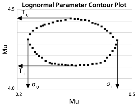
These points are represented graphically in the following contour plot:

(Note that this plot is generated with degrees of freedom [math]\displaystyle{ k=1\,\! }[/math], as we are only determining bounds on one parameter. The contour plots generated in Weibull++ are done with degrees of freedom [math]\displaystyle{ k=2\,\! }[/math], for use in comparing both parameters simultaneously.) As can be determined from the table the lowest calculated value for [math]\displaystyle{ {\mu }'\,\! }[/math] is 4.1145, while the highest is 4.4708. These represent the two-sided 75% confidence limits on this parameter. Since solutions for the equation do not exist for values of [math]\displaystyle{ {{\sigma' }}\,\! }[/math] below 0.24 or above 0.48, these can be considered the two-sided 75% confidence limits for this parameter. In order to obtain more accurate values for the confidence limits on [math]\displaystyle{ {{\sigma'}}\,\! }[/math], we can perform the same procedure as before, but finding the two values of [math]\displaystyle{ \sigma \,\! }[/math] that correspond with a given value of [math]\displaystyle{ {\mu }'.\,\! }[/math] Using this method, we find that the 75% confidence limits on [math]\displaystyle{ {{\sigma'}}\,\! }[/math] are 0.23405 and 0.48936, which are close to the initial estimates of 0.24 and 0.48.

Bounds on Time and Reliability

In order to calculate the bounds on a time estimate for a given reliability, or on a reliability estimate for a given time, the likelihood function needs to be rewritten in terms of one parameter and time/reliability, so that the maximum and minimum values of the time can be observed as the parameter is varied. This can be accomplished by substituting a form of the normal reliability equation into the likelihood function. The normal reliability equation can be written as:

[math]\displaystyle{ R=1-\Phi \left( \frac{\text{ln}(t)-{\mu }'}{{{\sigma'}}} \right)\,\! }[/math]

This can be rearranged to the form:

[math]\displaystyle{ {\mu }'=\text{ln}(t)-{{\sigma'}}\cdot {{\Phi }^{-1}}(1-R)\,\! }[/math]

where [math]\displaystyle{ {{\Phi }^{-1}}\,\! }[/math] is the inverse standard normal. This equation can now be substituted into likelihood function to produce a likelihood equation in terms of [math]\displaystyle{ {{\sigma'}},\,\! }[/math] [math]\displaystyle{ t\,\! }[/math] and [math]\displaystyle{ R\,\! }[/math]:

[math]\displaystyle{ L({{\sigma'}},t/R)=\underset{i=1}{\overset{N}{\mathop \prod }}\,\frac{1}{{{x}_{i}}\cdot {{\sigma'}}\cdot \sqrt{2\pi }}\cdot {{e}^{-\tfrac{1}{2}{{\left( \tfrac{\text{ln}({{x}_{i}})-\left( \text{ln}(t)-{{\sigma'}}\cdot {{\Phi }^{-1}}(1-R) \right)}{{{\sigma'}}} \right)}^{2}}}}\,\! }[/math]

The unknown variable [math]\displaystyle{ t/R\,\! }[/math] depends on what type of bounds are being determined. If one is trying to determine the bounds on time for a given reliability, then [math]\displaystyle{ R\,\! }[/math] is a known constant and [math]\displaystyle{ t\,\! }[/math] is the unknown variable. Conversely, if one is trying to determine the bounds on reliability for a given time, then [math]\displaystyle{ t\,\! }[/math] is a known constant and [math]\displaystyle{ R\,\! }[/math] is the unknown variable. Either way, the above equation can be used to solve the likelihood ratio equation for the values of interest.

Example: LR Bounds on Time

Lognormal Distribution Likelihood Ratio Bound Example (Time)

For the same data set given for the parameter bounds example, determine the two-sided 75% confidence bounds on the time estimate for a reliability of 80%. The ML estimate for the time at [math]\displaystyle{ R(t)=80%\,\! }[/math] is 55.718.

Solution

In this example, we are trying to determine the two-sided 75% confidence bounds on the time estimate of 55.718. This is accomplished by substituting [math]\displaystyle{ R=0.80\,\! }[/math] and [math]\displaystyle{ \alpha =0.75\,\! }[/math] into the likelihood function, and varying [math]\displaystyle{ {{\sigma' }}\,\! }[/math] until the maximum and minimum values of [math]\displaystyle{ t\,\! }[/math] are found. The following table gives the values of [math]\displaystyle{ t\,\! }[/math] based on given values of [math]\displaystyle{ {{\sigma' }}\,\! }[/math].

[math]\displaystyle{ \begin{matrix} {{\sigma' }} & {{t}_{1}} & {{t}_{2}} & {{\sigma' }} & {{t}_{1}} & {{t}_{2}} \\ 0.24 & 56.832 & 62.879 & 0.37 & 44.841 & 64.031 \\ 0.25 & 54.660 & 64.287 & 0.38 & 44.494 & 63.454 \\ 0.26 & 53.093 & 65.079 & 0.39 & 44.200 & 62.809 \\ 0.27 & 51.811 & 65.576 & 0.40 & 43.963 & 62.093 \\ 0.28 & 50.711 & 65.881 & 0.41 & 43.786 & 61.304 \\ 0.29 & 49.743 & 66.041 & 0.42 & 43.674 & 60.436 \\ 0.30 & 48.881 & 66.085 & 0.43 & 43.634 & 59.481 \\ 0.31 & 48.106 & 66.028 & 0.44 & 43.681 & 58.426 \\ 0.32 & 47.408 & 65.883 & 0.45 & 43.832 & 57.252 \\ 0.33 & 46.777 & 65.657 & 0.46 & 44.124 & 55.924 \\ 0.34 & 46.208 & 65.355 & 0.47 & 44.625 & 54.373 \\ 0.35 & 45.697 & 64.983 & 0.48 & 45.517 & 52.418 \\ 0.36 & 45.242 & 64.541 & {} & {} & {} \\ \end{matrix}\,\! }[/math]

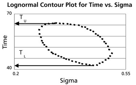
This data set is represented graphically in the following contour plot:

As can be determined from the table, the lowest calculated value for [math]\displaystyle{ t\,\! }[/math] is 43.634, while the highest is 66.085. These represent the two-sided 75% confidence limits on the time at which reliability is equal to 80%.

Example: LR Bounds on Reliability

Lognormal Distribution Likelihood Ratio Bound Example (Reliability)

For the same data set given above for the parameter bounds example, determine the two-sided 75% confidence bounds on the reliability estimate for [math]\displaystyle{ t=65\,\! }[/math]. The ML estimate for the reliability at [math]\displaystyle{ t=65\,\! }[/math] is 64.261%.

Solution

In this example, we are trying to determine the two-sided 75% confidence bounds on the reliability estimate of 64.261%. This is accomplished by substituting [math]\displaystyle{ t=65\,\! }[/math] and [math]\displaystyle{ \alpha =0.75\,\! }[/math] into the likelihood function, and varying [math]\displaystyle{ {{\sigma'}}\,\! }[/math] until the maximum and minimum values of [math]\displaystyle{ R\,\! }[/math] are found. The following table gives the values of [math]\displaystyle{ R\,\! }[/math] based on given values of [math]\displaystyle{ {{\sigma' }}\,\! }[/math].

[math]\displaystyle{ \begin{matrix} {{\sigma'}} & {{R}_{1}} & {{R}_{2}} & {{\sigma'}} & {{R}_{1}} & {{R}_{2}} \\ 0.24 & 61.107% & 75.910% & 0.37 & 43.573% & 78.845% \\ 0.25 & 55.906% & 78.742% & 0.38 & 43.807% & 78.180% \\ 0.26 & 55.528% & 80.131% & 0.39 & 44.147% & 77.448% \\ 0.27 & 50.067% & 80.903% & 0.40 & 44.593% & 76.646% \\ 0.28 & 48.206% & 81.319% & 0.41 & 45.146% & 75.767% \\ 0.29 & 46.779% & 81.499% & 0.42 & 45.813% & 74.802% \\ 0.30 & 45.685% & 81.508% & 0.43 & 46.604% & 73.737% \\ 0.31 & 44.857% & 81.387% & 0.44 & 47.538% & 72.551% \\ 0.32 & 44.250% & 81.159% & 0.45 & 48.645% & 71.212% \\ 0.33 & 43.827% & 80.842% & 0.46 & 49.980% & 69.661% \\ 0.34 & 43.565% & 80.446% & 0.47 & 51.652% & 67.789% \\ 0.35 & 43.444% & 79.979% & 0.48 & 53.956% & 65.299% \\ 0.36 & 43.450% & 79.444% & {} & {} & {} \\ \end{matrix}\,\! }[/math]

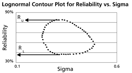
This data set is represented graphically in the following contour plot:

As can be determined from the table, the lowest calculated value for [math]\displaystyle{ R\,\! }[/math] is 43.444%, while the highest is 81.508%. These represent the two-sided 75% confidence limits on the reliability at [math]\displaystyle{ t=65\,\! }[/math].

Bayesian Confidence Bounds

Bounds on Parameters

From Parameter Estimation, we know that the marginal distribution of parameter [math]\displaystyle{ {\mu }'\,\! }[/math] is:

[math]\displaystyle{ \begin{align} f({\mu }'|Data)= & \int_{0}^{\infty }f({\mu }',{{\sigma'}}|Data)d{{\sigma'}} \\ = & \frac{\int_{0}^{\infty }L(Data|{\mu }',{{\sigma'}})\varphi ({\mu }')\varphi ({{\sigma'}})d{{\sigma'}}}{\int_{0}^{\infty }\int_{-\infty }^{\infty }L(Data|{\mu }',{{\sigma'}})\varphi ({\mu }')\varphi ({{\sigma'}})d{\mu }'d{{\sigma'}}} \end{align}\,\! }[/math]

where:

[math]\displaystyle{ \varphi ({{\sigma '}})\,\! }[/math] is [math]\displaystyle{ \tfrac{1}{{{\sigma '}}}\,\! }[/math], non-informative prior of [math]\displaystyle{ {{\sigma '}}\,\! }[/math].

[math]\displaystyle{ \varphi ({\mu }')\,\! }[/math] is an uniform distribution from - [math]\displaystyle{ \infty \,\! }[/math] to + [math]\displaystyle{ \infty \,\! }[/math], non-informative prior of [math]\displaystyle{ {\mu }'\,\! }[/math]. With the above prior distributions, [math]\displaystyle{ f({\mu }'|Data)\,\! }[/math] can be rewritten as:

[math]\displaystyle{ f({\mu }'|Data)=\frac{\int_{0}^{\infty }L(Data|{\mu }',{{\sigma '}})\tfrac{1}{{{\sigma '}}}d{{\sigma '}}}{\int_{0}^{\infty }\int_{-\infty }^{\infty }L(Data|{\mu }',{{\sigma '}})\tfrac{1}{{{\sigma '}}}d{\mu }'d{{\sigma '}}}\,\! }[/math]

The one-sided upper bound of [math]\displaystyle{ {\mu }'\,\! }[/math] is:

[math]\displaystyle{ CL=P({\mu }'\le \mu _{U}^{\prime })=\int_{-\infty }^{\mu _{U}^{\prime }}f({\mu }'|Data)d{\mu }'\,\! }[/math]

The one-sided lower bound of [math]\displaystyle{ {\mu }'\,\! }[/math] is:

[math]\displaystyle{ 1-CL=P({\mu }'\le \mu _{L}^{\prime })=\int_{-\infty }^{\mu _{L}^{\prime }}f({\mu }'|Data)d{\mu }'\,\! }[/math]

The two-sided bounds of [math]\displaystyle{ {\mu }'\,\! }[/math] is:

[math]\displaystyle{ CL=P(\mu _{L}^{\prime }\le {\mu }'\le \mu _{U}^{\prime })=\int_{\mu _{L}^{\prime }}^{\mu _{U}^{\prime }}f({\mu }'|Data)d{\mu }'\,\! }[/math]

The same method can be used to obtained the bounds of [math]\displaystyle{ {{\sigma '}}\,\! }[/math].

Bounds on Time (Type 1)

The reliable life of the lognormal distribution is:

[math]\displaystyle{ \begin{align} \ln T={\mu }'+{{\sigma '}}{{\Phi }^{-1}}(1-R) \end{align}\,\! }[/math]

The one-sided upper on time bound is given by:

[math]\displaystyle{ CL=\underset{}{\overset{}{\mathop{\Pr }}}\,(\ln t\le \ln {{t}_{U}})=\underset{}{\overset{}{\mathop{\Pr }}}\,({\mu }'+{{\sigma '}}{{\Phi }^{-1}}(1-R)\le \ln {{t}_{U}})\,\! }[/math]

The above equation can be rewritten in terms of [math]\displaystyle{ {\mu }'\,\! }[/math] as:

[math]\displaystyle{ CL=\underset{}{\overset{}{\mathop{\Pr }}}\,({\mu }'\le \ln {{t}_{U}}-{{\sigma '}}{{\Phi }^{-1}}(1-R)\,\! }[/math]

From the posterior distribution of [math]\displaystyle{ {\mu }'\,\! }[/math] get:

[math]\displaystyle{ CL=\frac{\int_{0}^{\infty }\int_{-\infty }^{\ln {{t}_{U}}-{{\sigma'}}{{\Phi }^{-1}}(1-R)}L({{\sigma '}},{\mu }')\tfrac{1}{{{\sigma '}}}d{\mu }'d{{\sigma '}}}{\int_{0}^{\infty }\int_{-\infty }^{\infty }L({{\sigma '}},{\mu }')\tfrac{1}{{{\sigma '}}}d{\mu }'d{{\sigma '}}}\,\! }[/math]

The above equation is solved w.r.t. [math]\displaystyle{ {{t}_{U}}.\,\! }[/math] The same method can be applied for one-sided lower bounds and two-sided bounds on Time.

Bounds on Reliability (Type 2)

The one-sided upper bound on reliability is given by:

[math]\displaystyle{ CL=\underset{}{\overset{}{\mathop{\Pr }}}\,(R\le {{R}_{U}})=\underset{}{\overset{}{\mathop{\Pr }}}\,({\mu }'\le \ln t-{{\sigma '}}{{\Phi }^{-1}}(1-{{R}_{U}}))\,\! }[/math]

From the posterior distribution of [math]\displaystyle{ {\mu }'\,\! }[/math] is:

[math]\displaystyle{ CL=\frac{\int_{0}^{\infty }\int_{-\infty }^{\ln t-{{\sigma '}}{{\Phi }^{-1}}(1-{{R}_{U}})}L({{\sigma'}},{\mu }')\tfrac{1}{{{\sigma'}}}d{\mu }'d{{\sigma '}}}{\int_{0}^{\infty }\int_{-\infty }^{\infty }L({{\sigma '}},{\mu }')\tfrac{1}{{{\sigma '}}}d{\mu }'d{{\sigma '}}}\,\! }[/math]

The above equation is solved w.r.t. [math]\displaystyle{ {{R}_{U}}.\,\! }[/math] The same method is used to calculate the one-sided lower bounds and two-sided bounds on Reliability.

Example: Bayesian Bounds

Lognormal Distribution Bayesian Bound Example (Parameters)

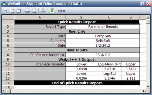
Determine the two-sided 90% Bayesian confidence bounds on the lognormal parameter estimates for the data given next:

Data Point Index	State End Time
1	2
2	5
3	11
4	23
5	29
6	37
7	43
8	59

Solution

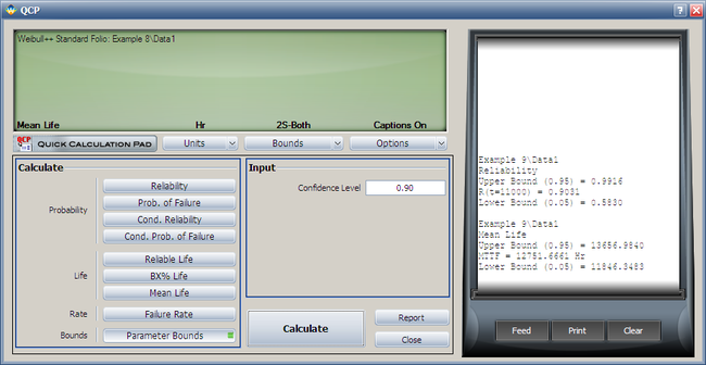
The data points are entered into a times-to-failure data sheet. The lognormal distribution is selected under Distributions. The Bayesian confidence bounds method only applies for the MLE analysis method, therefore, Maximum Likelihood (MLE) is selected under Analysis Method and Use Bayesian is selected under the Confidence Bounds Method in the Analysis tab.

The two-sided 90% Bayesian confidence bounds on the lognormal parameter are obtained using the QCP and clicking on the Calculate Bounds button in the Parameter Bounds tab as follows: