Inverse Power Law (IPL)-Lognormal Model
New format available! This reference is now available in a new format that offers faster page load, improved display for calculations and images and more targeted search.
As of January 2024, this Reliawiki page will not continue to be updated. Please update all links and bookmarks to the latest references at ALTA examples and ALTA reference examples.
|
Inverse Power Law (IPL)-Lognormal Model |
This example validates the calculations for the IPL life stress relationship with a lognormal distribution in ALTA standard folios.
Reference Case
The data set is from Example 19.10 on page 504 in book Statistical Methods for Reliability Data by Dr. Meeker and Dr. Escobar, John Wiley & Sons, 1998.
Data
A Mylar-Polyurethane insulating structure was tested under several different voltage settings. The following table shows the test data.
| Time Failed (Hr) | Voltage (kV) |
|---|---|
| 15 | 219 |
| 16 | 219 |
| 36 | 219 |
| 50 | 219 |
| 55 | 219 |
| 95 | 219 |
| 122 | 219 |
| 129 | 219 |
| 625 | 219 |
| 700 | 219 |
| 49 | 157.1 |
| 99 | 157.1 |
| 154.5 | 157.1 |
| 180 | 157.1 |
| 291 | 157.1 |
| 447 | 157.1 |
| 510 | 157.1 |
| 600 | 157.1 |
| 1656 | 157.1 |
| 1721 | 157.1 |
| 188 | 122.4 |
| 297 | 122.4 |
| 405 | 122.4 |
| 744 | 122.4 |
| 1218 | 122.4 |
| 1340 | 122.4 |
| 1715 | 122.4 |
| 3382 | 122.4 |
| 606 | 100.3 |
| 1012 | 100.3 |
| 2520 | 100.3 |
| 2610 | 100.3 |
| 3988 | 100.3 |
| 4100 | 100.3 |
| 5025 | 100.3 |
| 6842 | 100.3 |
Result
The following function is used for the Ln-Mean [math]\displaystyle{ \,\!\mu {}' }[/math]:
- [math]\displaystyle{ \,\!\mu {}'=\beta _{0}+\beta _{1}\times log\left ( V \right ) }[/math]
where V is the voltage and its natural log transform is used in the above life stress relation.
This function can be written in the following way:
- [math]\displaystyle{ \,\!e^{\mu {}'}=e^{\alpha _{0}+\alpha _{1}log\left ( V \right )} }[/math]
The above equation is the general log-linear model in ALTA. In ALTA, the coefficients are denoted by [math]\displaystyle{ \,\!\alpha _{i} }[/math].
In fact, the above model also can be expressed using the traditional IPL (inverse power law) model:
- [math]\displaystyle{ \,\!e^{\mu {}'}=\frac{1}{K\cdot V^{n}} }[/math]
where [math]\displaystyle{ \,\!K=e^{-\alpha _{0}} }[/math] and [math]\displaystyle{ \,\!n=-\alpha _{1} }[/math].
In the book, the following results are provided:
- ML estimations for the model parameters are: [math]\displaystyle{ \,\!\sigma =1.05 }[/math] , [math]\displaystyle{ \,\!\beta _{0}=27.5 }[/math] and [math]\displaystyle{ \,\!\beta _{1}=-4.29 }[/math].
- The standard deviation of each parameter are: [math]\displaystyle{ \,\!std\left ( \sigma \right )=0.12 }[/math] , [math]\displaystyle{ \,\!std\left ( \beta _{0} \right )=3.0 }[/math] and [math]\displaystyle{ \,\!std\left ( \beta _{1} \right )=0.6 }[/math].
- Therefore, their variances are: [math]\displaystyle{ \,\!Var\left ( \sigma \right )=0.0144 }[/math] , [math]\displaystyle{ \,\!Var\left ( \beta _{0} \right )=9 }[/math] and [math]\displaystyle{ \,\!Var\left ( \beta _{1} \right )=0.36 }[/math].
- The log-likelihood value is -271.4.
- The 95% two-sided confidence intervals are: for [math]\displaystyle{ \,\!\sigma }[/math] , it is [0.83, 1.32]; for [math]\displaystyle{ \,\!\beta _{0} }[/math] , it is [21.6, 33.4]; and for [math]\displaystyle{ \,\!\beta _{1} }[/math] , it is [-5.46, -3.11].
Results in ALTA
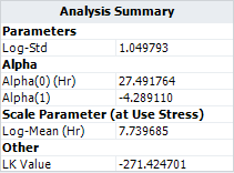
- ML estimations for the model parameters are:
- The variance and covariance matrix for model parameters is:
- The log-likelihood value is -271.4247.
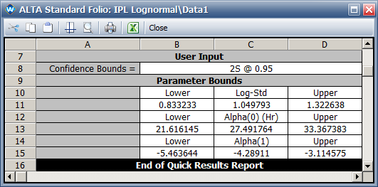
- The 95% two-sided confidence intervals are:


