Growth Plan for Four Phases
New format available! This reference is now available in a new format that offers faster page load, improved display for calculations and images and more targeted search.
As of January 2024, this Reliawiki page will not continue to be updated. Please update all links and bookmarks to the latest references at RGA examples and RGA reference examples.
This example appears in the Reliability growth reference.
The reliability team of a product manufacturer has put together a reliability growth plan, based on the Crow Extended model, for one of their new products. The reliability growth model was constructed with the following inputs:
- The requirement or goal MTBF is [math]\displaystyle{ {{M}_{G}}=910\,\! }[/math] hours.
- The growth potential design margin factor is [math]\displaystyle{ GPDM=1.35\,\! }[/math].
- The average effectiveness factor is [math]\displaystyle{ d\quad =0.7.\,\! }[/math]
- The management strategy is [math]\displaystyle{ msr=0.95\,\! }[/math].
- The beta parameter for the discovery function, [math]\displaystyle{ h\left( t \right),\,\! }[/math] of the type B failure modes is [math]\displaystyle{ \beta =0.70\,\! }[/math].
- The test is planned to be conducted in four phases. The cumulative phase end times are [math]\displaystyle{ {{T}_{1}}=19000,{{T}_{2}}=38000\,\! }[/math], [math]\displaystyle{ {{T}_{3}}=70000\,\! }[/math] and [math]\displaystyle{ {{T}_{4}}=100000\,\! }[/math]. The average fix delay in terms of test hours for each phase is: [math]\displaystyle{ {{L}_{1}}=10000\,\! }[/math], [math]\displaystyle{ {{L}_{2}}=15000,\,\! }[/math] [math]\displaystyle{ {{L}_{3}}=20000\,\! }[/math] and [math]\displaystyle{ {{L}_{4}}=25000\,\! }[/math] hours.
Determine the following:
- Plot the nominal and actual reliability growth curves for this program, using the RGA software.
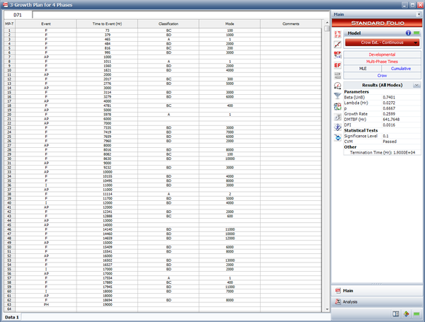
- The reliability program was initiated and actual test data from phase 1 is now available. The test data were analyzed using the Crow Extended - Continuous Evaluation model and the following figure shows the results.
Note that the I events, which represent the times for implementation of fixes for BD modes, occur at least 10,000 hours after the first occurrence of the specific BD mode. This is a reflection of the average fix delay being equal to 10,000 hours for the first test phase. Of course we could have some exceptions that could have been fixed before 10,000 hours after the first occurrence (i.e., discovery) of the mode, but on average, they should be fixed after 10,000 hours.
The same applies to the delayed fixes at the end of phase 1. On average there should be at least 10,000 test hours between the discovery of the failure mode and the implementation of a fix for that mode, so failure modes discovered after 9,000 hours of testing in the first phase cannot be implemented at the end of the first phase.
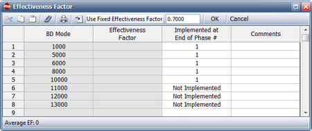
The figure below shows the effectiveness factor window. The record shows that the fixes for failure modes BD 11000, BD 12000 and BD 13000 are not implemented at the end of the first phase due to the fix delay. The effectiveness factor used is in accordance with the planning model and has been fixed to 0.7.
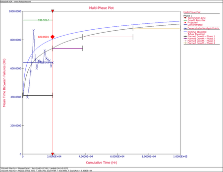
Construct a multi-phase graph that shows the analysis points for the test data in phase 1, as compared to the nominal and actual idealized growth curves for this reliability growth plan. Is the program on track, so far, as compared to the plan?
Solution
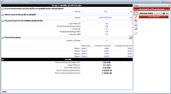
- The following figures show the plan inputs, phase durations and average fix delays as entered in RGA's continuous growth planning folio, together with the results of the growth model.
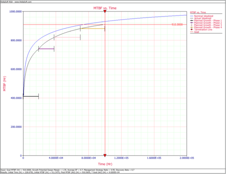
The next figure shows the nominal and actual idealized growth curves for this program, together with the program MTBF goal.
- The next step is to associate the reliability growth plan with the data from phase 1. To do that, right-click the Multiplots heading in the current project explorer and choose Add Multi-Phase Plot from the shortcut menu, then follow the wizard to specify the data sheet that contains the phase 1 data with the folio that defines the growth plan. The figure below shows the generated multi-phase plot, which brings together the reliability growth planning model with the actual test results. This plot shows the demonstrated MTBF for each analysis point during the first phase of testing. Analysis points for projected and growth potential MTBF can also be plotted. For this example, it can be said that the program is on track since the demonstrated MTBF of the first phase is higher than the planned MTBF for that phase.
The multi-phase plot can be updated continuously as the growth program progresses and more test data become available. In that manner, the reliability team can assess the actual reliability performance against the established goals.

