Gompertz Model Examples
 |
New format available! This reference is now available in a new format that offers faster page load, improved display for calculations and images and more targeted search.
As of January 2024, this Reliawiki page will not continue to be updated. Please update all links and bookmarks to the latest references at RGA examples and RGA reference examples.
These examples appear in the Reliability growth reference.
Parameter Estimation
Standard Gompertz Model
A device is required to have a reliability of 92% at the end of a 12-month design and development period. The following table gives the data obtained for the first five moths.
- What will the reliability be at the end of this 12-month period?
- What will the maximum achievable reliability be if the reliability program plan pursued during the first 5 months is continued?
- How do the predicted reliability values compare with the actual values?
| Group Number | Growth Time [math]\displaystyle{ T\,\! }[/math](months) | Reliability [math]\displaystyle{ R\,\! }[/math](%) | [math]\displaystyle{ \ln{R}\,\! }[/math] |
|---|---|---|---|
| 0 | 58 | 4.060 | |
| 1 | 1 | 66 | 4.190 |
| [math]\displaystyle{ {{S}_{1}}\,\! }[/math] = 8.250 | |||
| 2 | 72.5 | 4.284 | |
| 2 | 3 | 78 | 4.357 |
| [math]\displaystyle{ {{S}_{2}}\,\! }[/math] = 8.641 | |||
| 4 | 82 | 4.407 | |
| 3 | 5 | 85 | 4.443 |
| [math]\displaystyle{ {{S}_{3}}\,\! }[/math] = 8.850 |
Solution
After generating the table above and calculating the last column to find [math]\displaystyle{ {{S}_{1}}\,\! }[/math], [math]\displaystyle{ {{S}_{2}}\,\! }[/math] and [math]\displaystyle{ {{S}_{3}}\,\! }[/math], proceed as follows:
- Solve for the value of [math]\displaystyle{ c\,\! }[/math]:
- [math]\displaystyle{ \begin{align} c= & {{\left( \frac{8.850-8.641}{8.641-8.250} \right)}^{\tfrac{1}{2}}} \\ = & 0.731 \end{align}\,\! }[/math]
- Solve for the value of [math]\displaystyle{ a\,\! }[/math]:
- [math]\displaystyle{ \begin{align} a&=e^\left[({\frac{1}{2}\left ( 8.250+\frac{S_{2}-S_{1}}{1-c^{n\cdot 1}} \right )} \right ] \\ &=e^{4.545} \\ &=94.16% \end{align}\,\! }[/math]
- This is the upper limit for the reliability as [math]\displaystyle{ T\to \infty \,\! }[/math].
- Solve for the value of [math]\displaystyle{ b\,\! }[/math]:
- [math]\displaystyle{ \begin{align} b= & {{e}^{\left[ \tfrac{(8.641-8.250)(0.731-1)}{{{(1-{{0.731}^{2}})}^{2}}} \right]}} \\ = & {{e}^{(-0.485)}} \\ = & 0.615 \end{align}\,\! }[/math]
Now, that the initial values have been determined, the Gauss-Newton method can be used. Therefore, substituting [math]\displaystyle{ {{Y}_{i}}={{R}_{i}},\,\! }[/math] [math]\displaystyle{ g_{1}^{(0)}=94.16,\,\! }[/math] [math]\displaystyle{ g_{2}^{(0)}=0.615,\,\! }[/math] [math]\displaystyle{ g_{3}^{(0)}=0.731,\,\! }[/math] [math]\displaystyle{ {{Y}^{(0)}},{{D}^{(0)}},\,\! }[/math] [math]\displaystyle{ {{\nu }^{(0)}}\,\! }[/math] become:
- [math]\displaystyle{ {{Y}^{(0)}}=\left[ \begin{matrix} 0.0916 \\ 0.0015 \\ -0.1190 \\ 0.1250 \\ 0.0439 \\ -0.0743 \\ \end{matrix} \right]\,\! }[/math]
- [math]\displaystyle{ {{D}^{(0)}}=\left[ \begin{matrix} 0.6150 & 94.1600 & 0.0000 \\ 0.7009 & 78.4470 & -32.0841 \\ 0.7712 & 63.0971 & -51.6122 \\ 0.8270 & 49.4623 & -60.6888 \\ 0.8704 & 38.0519 & -62.2513 \\ 0.9035 & 28.8742 & -59.0463 \\ \end{matrix} \right]\,\! }[/math]
- [math]\displaystyle{ {{\nu }^{(0)}}=\left[ \begin{matrix} g_{1}^{(0)} \\ g_{2}^{(0)} \\ g_{3}^{(0)} \\ \end{matrix} \right]=\left[ \begin{matrix} 94.16 \\ 0.615 \\ 0.731 \\ \end{matrix} \right]\,\! }[/math]
The estimate of the parameters [math]\displaystyle{ {{\nu }^{(0)}}\,\! }[/math] is given by:
- [math]\displaystyle{ \begin{align} \hat{v}&=\left ( D^{(0)}D^{(0)} \right )^{-1}D^{(0)}Y^{(0)} \\ &=\begin{bmatrix}0.061575\\ 0.000222\\ 0.001123\end{bmatrix} \end{align} }[/math]
The revised estimated regression coefficients in matrix form are:
- [math]\displaystyle{ \begin{align} g^{(1)}&=g^{(0)} + \hat{v}^{(0)} \\ &= \begin{bmatrix}94.16\\ 0.615\\ 0.731\end{bmatrix}+\begin{bmatrix}0.061575\\ 0.000222\\ 0.001123\end{bmatrix} \\ &=\begin{bmatrix}94.2216\\ 0.6152\\ 0.7321\end{bmatrix} \end{align} }[/math]
If the Gauss-Newton method works effectively, then the relationship [math]\displaystyle{ {{Q}^{(k+1)}}\lt {{Q}^{(k)}}\,\! }[/math] has to hold, meaning that [math]\displaystyle{ {{g}^{(k+1)}}\,\! }[/math] gives better estimates than [math]\displaystyle{ {{g}^{(k)}}\,\! }[/math], after [math]\displaystyle{ k\,\! }[/math]. With the starting coefficients, [math]\displaystyle{ {{g}^{(0)}}\,\! }[/math], [math]\displaystyle{ Q\,\! }[/math] is:
- [math]\displaystyle{ \begin{align} Q^{0}&=\sum_{i=1}^{N}\left [ Y_{i}-f\left ( T_{i}, g^{(0)} \right ) \right ]^{2}\\ &= 0.045622 \end{align} }[/math]
And with the coefficients at the end of the first iteration, [math]\displaystyle{ {{g}^{(1)}}\,\! }[/math], [math]\displaystyle{ Q\,\! }[/math] is:
- [math]\displaystyle{ \begin{align} Q^{1}&=\sum_{i=1}^{N}\left [ Y_{i}-f\left ( T_{i}, g^{(1)} \right ) \right ]^{2}\\ &= 0.041439 \end{align} }[/math]
Therefore, it can be justified that the Gauss-Newton method works in the right direction. The iterations are continued until the relationship [math]\displaystyle{ Q^{(s-1)}-Q^{(s)}\simeq 0 }[/math] is satisfied. Note that the RGA software uses a different analysis method called the Levenberg-Marquardt. This method utilizes the best features of the Gauss-Newton method and the method of the steepest descent, and occupies a middle ground between these two methods. The estimated parameters using RGA are shown in the figure below.

They are:
- [math]\displaystyle{ \begin{align} & \widehat{a}= & 0.9422 \\ & \widehat{b}= & 0.6152 \\ & \widehat{c}= & 0.7321 \end{align}\,\! }[/math]
The Gompertz reliability growth curve is:
- [math]\displaystyle{ R=0.9422{{(0.6152)}^{{{0.7321}^{T}}}}\,\! }[/math]
- The achievable reliability at the end of the 12-month period of design and development is:
- [math]\displaystyle{ \begin{align} R&=0.9422(0.6152)^{0.7321} &=0.9314 \end{align}\,\! }[/math]
- The maximum achievable reliability from Step 2, or from the value of [math]\displaystyle{ a\,\! }[/math], is 0.9422.
- The predicted reliability values, as calculated from the standard Gompertz model, are compared with the actual data in the table below. It may be seen in the table that the Gompertz curve appears to provide a very good fit for the data used because the equation reproduces the available data with less than 1% error. The standard Gompertz model is plotted in the figure below the table. The plot identifies the type of reliability growth curve that the equation represents.
Comparison of the Predicted Reliabilities with the Actual Data Growth Time [math]\displaystyle{ T\,\! }[/math](months) Gompertz Reliability(%) Raw Data Reliability(%) 0 57.97 58.00 1 66.02 66.00 2 72.62 72.50 3 77.87 78.00 4 81.95 82.00 5 85.07 85.00 6 87.43 7 89.20 8 90.52 9 91.50 10 92.22 11 92.75 12 93.14 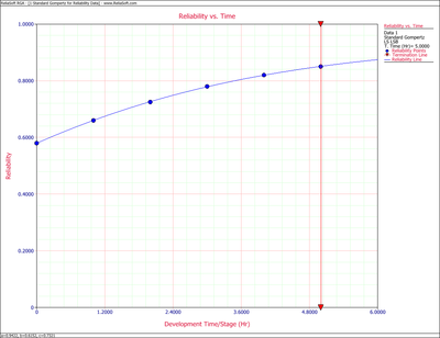

Modified Gompertz Model
A reliability growth data set is given in columns 1 and 2 of the following table. Find the modified Gompertz curve that represents the data and plot it comparatively with the raw data.
| Time(months) | Raw Data Reliability(%) | Gompertz Reliability(%) | Logistic Reliability(%) | Modified Gompertz Reliability(%) |
|---|---|---|---|---|
| 0 | 31.00 | 25.17 | 22.70 | 31.18 |
| 1 | 35.50 | 38.33 | 38.10 | 35.08 |
| 2 | 49.30 | 51.35 | 56.40 | 49.92 |
| 3 | 70.10 | 62.92 | 73.00 | 69.23 |
| 4 | 83.00 | 72.47 | 85.00 | 83.72 |
| 5 | 92.20 | 79.94 | 93.20 | 92.06 |
| 6 | 96.40 | 85.59 | 96.10 | 96.29 |
| 7 | 98.60 | 89.75 | 98.10 | 98.32 |
| 8 | 99.00 | 92.76 | 99.10 | 99.27 |
Solution
To determine the parameters of the modified Gompertz curve, use:
- [math]\displaystyle{ \begin{align} & {{S}_{1}}(d)= & \underset{i=0}{\overset{2}{\mathop \sum }}\,\ln ({{R}_{oi}}-d) \\ & {{S}_{2}}(d)= & \underset{i=3}{\overset{5}{\mathop \sum }}\,\ln ({{R}_{oi}}-d) \\ & {{S}_{3}}(d)= & \underset{i=6}{\overset{8}{\mathop \sum }}\,\ln ({{R}_{oi}}-d) \end{align}\,\! }[/math]
- [math]\displaystyle{ c(d)={{\left[ \frac{{{S}_{3}}(d)-{{S}_{2}}(d)}{{{S}_{2}}(d)-{{S}_{1}}(d)} \right]}^{\tfrac{1}{3}}}\,\! }[/math]
- [math]\displaystyle{ a(d)={{e}^{\left[ \tfrac{1}{3}\left( {{S}_{1}}(d)+\tfrac{{{S}_{2}}(d)-{{S}_{1}}(d)}{1-{{[c(d)]}^{3}}} \right) \right]}}\,\! }[/math]
- [math]\displaystyle{ b(d)={{e}^{\left[ \tfrac{({{S}_{2}}(d)-{{S}_{1}}(d))(c(d)-1)}{{{\left[ 1-{{[c(d)]}^{3}} \right]}^{2}}} \right]}}\,\! }[/math]
and:
- [math]\displaystyle{ {{R}_{0}}=d+a(d)\cdot b(d)\,\! }[/math]
for [math]\displaystyle{ {{R}_{0}}=31%\,\! }[/math], the equation above may be rewritten as:
- [math]\displaystyle{ d-31+a(d)\cdot b(d)=0\,\! }[/math]
The equations for parameters [math]\displaystyle{ c\,\! }[/math], [math]\displaystyle{ a\,\! }[/math] and [math]\displaystyle{ b\,\! }[/math] can now be solved simultaneously. One method for solving these equations numerically is to substitute different values of [math]\displaystyle{ d\,\! }[/math], which must be less than [math]\displaystyle{ {{R}_{0}}\,\! }[/math], into the last equation shown above, and plot the results along the y-axis with the value of [math]\displaystyle{ d\,\! }[/math] along the x-axis. The value of [math]\displaystyle{ d\,\! }[/math] can then be read from the x-intercept. This can be repeated for greater accuracy using smaller and smaller increments of [math]\displaystyle{ d\,\! }[/math]. Once the desired accuracy on [math]\displaystyle{ d\,\! }[/math] has been achieved, the value of [math]\displaystyle{ d\,\! }[/math] can then be used to solve for [math]\displaystyle{ a\,\! }[/math], [math]\displaystyle{ b\,\! }[/math] and [math]\displaystyle{ c\,\! }[/math]. For this case, the initial estimates of the parameters are:
- [math]\displaystyle{ \begin{align} \widehat{a}= & 69.324 \\ \widehat{b}= & 0.002524 \\ \widehat{c}= & 0.46012 \\ \widehat{d}= & 30.825 \end{align}\,\! }[/math]
Now, since the initial values have been determined, the Gauss-Newton method can be used. Therefore, substituting [math]\displaystyle{ {{Y}_{i}}={{R}_{i}},\,\! }[/math] [math]\displaystyle{ g_{1}^{(0)}=69.324,\,\! }[/math] [math]\displaystyle{ g_{2}^{(0)}=0.002524,\,\! }[/math] [math]\displaystyle{ g_{3}^{(0)}=0.46012,\,\! }[/math] and [math]\displaystyle{ g_{4}^{(0)}=30.825\,\! }[/math], [math]\displaystyle{ {{Y}^{(0)}},{{D}^{(0)}},\,\! }[/math] [math]\displaystyle{ {{\nu }^{(0)}}\,\! }[/math] become:
- [math]\displaystyle{ {{Y}^{(0)}}=\left[ \begin{matrix} 0.000026 \\ 0.253873 \\ -1.062940 \\ 0.565690 \\ -0.845260 \\ 0.096737 \\ 0.076450 \\ 0.238155 \\ -0.320890 \\ \end{matrix} \right]\,\! }[/math]
- [math]\displaystyle{ {{D}^{(0)}}=\left[ \begin{matrix} 0.002524 & 69.3240 & 0.0000 & 1 \\ 0.063775 & 805.962 & -26.4468 & 1 \\ 0.281835 & 1638.82 & -107.552 & 1 \\ 0.558383 & 1493.96 & -147.068 & 1 \\ 0.764818 & 941.536 & -123.582 & 1 \\ 0.883940 & 500.694 & -82.1487 & 1 \\ 0.944818 & 246.246 & -48.4818 & 1 \\ 0.974220 & 116.829 & -26.8352 & 1 \\ 0.988055 & 54.5185 & -14.3117 & 1 \\ \end{matrix} \right]\,\! }[/math]
- [math]\displaystyle{ {{\nu }^{(0)}}=\left[ \begin{matrix} g_{1}^{(0)} \\ g_{2}^{(0)} \\ g_{3}^{(0)} \\ g_{4}^{(0)} \\ \end{matrix} \right]=\left[ \begin{matrix} 69.324 \\ 0.002524 \\ 0.46012 \\ 30.825 \\ \end{matrix} \right]\,\! }[/math]
The estimate of the parameters [math]\displaystyle{ {{\nu }^{(0)}}\,\! }[/math] is given by:
- [math]\displaystyle{ \begin{align} {{\widehat{\nu }}^{(0)}}= & {{\left( {{D}^{{{(0)}^{T}}}}{{D}^{(0)}} \right)}^{-1}}{{D}^{{{(0)}^{T}}}}{{Y}^{(0)}} \\ = & \left[ \begin{matrix} -0.275569 \\ -0.000549 \\ -0.003202 \\ 0.209458 \\ \end{matrix} \right] \end{align}\,\! }[/math]
The revised estimated regression coefficients in matrix form are given by:
- [math]\displaystyle{ \begin{align} {{g}^{(1)}}= & {{g}^{(0)}}+{{\widehat{\nu }}^{(0)}}. \\ = & \left[ \begin{matrix} 69.324 \\ 0.002524 \\ 0.46012 \\ 30.825 \\ \end{matrix} \right]+\left[ \begin{matrix} -0.275569 \\ -0.000549 \\ -0.003202 \\ 0.209458 \\ \end{matrix} \right] \\ = & \left[ \begin{matrix} 69.0484 \\ 0.00198 \\ 0.45692 \\ 31.0345 \\ \end{matrix} \right] \end{align}\,\! }[/math]
With the starting coefficients [math]\displaystyle{ {{g}^{(0)}}\,\! }[/math], [math]\displaystyle{ Q\,\! }[/math] is:
- [math]\displaystyle{ \begin{align} {{Q}^{(0)}}= & \underset{i=1}{\overset{N}{\mathop \sum }}\,{{\left( {{Y}_{i}}-f({{T}_{i}},{{g}^{(0)}}) \right)}^{2}} \\ = & 2.403672 \end{align}\,\! }[/math]
With the coefficients at the end of the first iteration, [math]\displaystyle{ {{g}^{(1)}}\,\! }[/math], [math]\displaystyle{ Q\,\! }[/math] is:
- [math]\displaystyle{ \begin{align} {{Q}^{(1)}}= & \underset{i=1}{\overset{N}{\mathop \sum }}\,{{\left[ {{Y}_{i}}-f\left( {{T}_{i}},{{g}^{(1)}} \right) \right]}^{2}} \\ = & 2.073964 \end{align}\,\! }[/math]
Therefore:
- [math]\displaystyle{ \begin{align} {{Q}^{(1)}}\lt {{Q}^{(0)}} \end{align}\,\! }[/math]
Hence, the Gauss-Newton method works in the right direction. The iterations are continued until the relationship of [math]\displaystyle{ {{Q}^{(s-1)}}-{{Q}^{(s)}}\simeq 0\,\! }[/math] has been satisfied. Using RGA, the estimators of the parameters are:
- [math]\displaystyle{ \begin{align} \widehat{a}= & 0.6904 \\ \widehat{b}= & 0.0020 \\ \widehat{c}= & 0.4567 \\ \widehat{d}= & 0.3104 \end{align}\,\! }[/math]
Therefore, the modified Gompertz model is:
- [math]\displaystyle{ R=0.3104+(0.6904){{(0.0020)}^{{{0.4567}^{T}}}}\,\! }[/math]
Using this equation, the predicted reliability is plotted in the following figure along with the raw data. As you can see, the modified Gompertz curve represents the data very well.

Comparing the Standard and Modified Gompertz Models
Using the data in the following table, determine whether the standard Gompertz or modified Gompertz would be better suited for analyzing the given data.
| Stage | Reliability (%) |
|---|---|
| 0 | 36 |
| 1 | 38 |
| 2 | 46 |
| 3 | 58 |
| 4 | 71 |
| 5 | 80 |
| 6 | 86 |
| 7 | 88 |
| 8 | 90 |
| 9 | 91 |
Solution
The standard Gompertz Reliability vs. Time plot is shown next.

The standard Gompertz seems to do a fairly good job of modeling the data. However, it appears that it is having difficulty modeling the S-shape of the data. The modified Gompertz Reliability vs. Time plot is shown next. As expected, the modified Gompertz does a much better job of handling the S-shape presented by the data and provides a better fit for this data.

Discrete Sequential Data Example
Calculate the parameters of the Gompertz model using the sequential data in the following table.
| Run Number | Result | Successes | Observed Reliability(%) |
|---|---|---|---|
| 1 | F | 0 | |
| 2 | F | 0 | |
| 3 | F | 0 | |
| 4 | S | 1 | 25.00 |
| 5 | F | 1 | 20.00 |
| 6 | F | 1 | 16.67 |
| 7 | S | 2 | 28.57 |
| 8 | S | 3 | 37.50 |
| 9 | S | 4 | 44.44 |
| 10 | S | 5 | 50.00 |
| 11 | S | 6 | 54.55 |
| 12 | S | 7 | 58.33 |
| 13 | S | 8 | 61.54 |
| 14 | S | 9 | 64.29 |
| 15 | S | 10 | 66.67 |
| 16 | S | 11 | 68.75 |
| 17 | F | 11 | 64.71 |
| 18 | S | 12 | 66.67 |
| 19 | F | 12 | 63.16 |
| 20 | S | 13 | 65.00 |
| 21 | S | 14 | 66.67 |
| 22 | S | 15 | 68.18 |
Solution
Using RGA, the parameter estimates are shown in the following figure.

Discrete Data - Grouped per Configuration Example
A new design is put through a reliability growth test. The requirement is that after the ninth stage the design will exhibit an 85% reliability with a 90% confidence level. Given the data in the following table, do the following:
- Estimate the parameters of the standard Gompertz model.
- What is the initial reliability at [math]\displaystyle{ T=0\,\! }[/math] ?
- Determine the reliability at the end of the ninth stage and check to see whether the goal has been met.
| Stage | Number of Units | Number of Failures |
|---|---|---|
| 1 | 10 | 5 |
| 2 | 8 | 3 |
| 3 | 9 | 3 |
| 4 | 9 | 2 |
| 5 | 10 | 2 |
| 6 | 10 | 1 |
| 7 | 10 | 1 |
| 8 | 10 | 1 |
| 9 | 10 | 1 |
Solution
- The data is entered in cumulative format and the estimated standard Gompertz parameters are shown in the following figure.
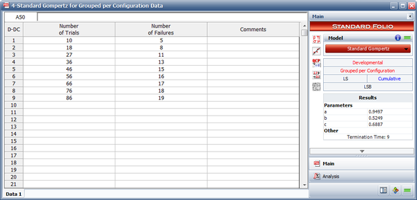
- The initial reliability at [math]\displaystyle{ T=0\,\! }[/math] is equal to:
- [math]\displaystyle{ \begin{align} {{R}_{T=0}}= & a\cdot b \\ = & 0.9497\cdot 0.5249 \\ = & 0.4985 \end{align}\,\! }[/math]
- The reliability at the ninth stage can be calculated using the Quick Calculation Pad (QCP) as shown in the figure below.
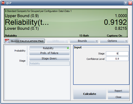
The estimated reliability at the end of the ninth stage is equal to 91.92%. However, the lower limit at the 90% 1-sided confidence bound is equal to 82.15%. Therefore, the required goal of 85% reliability at a 90% confidence level has not been met.

