Crow-AMSAA Model Examples
 |
New format available! This reference is now available in a new format that offers faster page load, improved display for calculations and images and more targeted search.
As of January 2024, this Reliawiki page will not continue to be updated. Please update all links and bookmarks to the latest references at RGA examples and RGA reference examples.
These examples appear in the Reliability growth reference.
Parameter Estimation Examples
Parameter Estimation for Failure Times Data
A prototype of a system was tested with design changes incorporated during the test. The following table presents the data collected over the entire test. Find the Crow-AMSAA parameters and the intensity function using maximum likelihood estimators.
| Row | Time to Event (hr) | [math]\displaystyle{ ln{(T)}\,\! }[/math] |
|---|---|---|
| 1 | 2.7 | 0.99325 |
| 2 | 10.3 | 2.33214 |
| 3 | 12.5 | 2.52573 |
| 4 | 30.6 | 3.42100 |
| 5 | 57.0 | 4.04305 |
| 6 | 61.3 | 4.11578 |
| 7 | 80.0 | 4.38203 |
| 8 | 109.5 | 4.69592 |
| 9 | 125.0 | 4.82831 |
| 10 | 128.6 | 4.85671 |
| 11 | 143.8 | 4.96842 |
| 12 | 167.9 | 5.12337 |
| 13 | 229.2 | 5.43459 |
| 14 | 296.7 | 5.69272 |
| 15 | 320.6 | 5.77019 |
| 16 | 328.2 | 5.79362 |
| 17 | 366.2 | 5.90318 |
| 18 | 396.7 | 5.98318 |
| 19 | 421.1 | 6.04287 |
| 20 | 438.2 | 6.08268 |
| 21 | 501.2 | 6.21701 |
| 22 | 620.0 | 6.42972 |
Solution
For the failure terminated test, [math]\displaystyle{ {\beta}\,\! }[/math] is:
- [math]\displaystyle{ \begin{align} \widehat{\beta }&=\frac{n}{n\ln {{T}^{*}}-\underset{i=1}{\overset{n}{\mathop{\sum }}}\,\ln {{T}_{i}}} \\ &=\frac{22}{22\ln 620-\underset{i=1}{\overset{22}{\mathop{\sum }}}\,\ln {{T}_{i}}} \\ \end{align}\,\! }[/math]
where:
- [math]\displaystyle{ \underset{i=1}{\overset{22}{\mathop \sum }}\,\ln {{T}_{i}}=105.6355\,\! }[/math]
Then:
- [math]\displaystyle{ \widehat{\beta }=\frac{22}{22\ln 620-105.6355}=0.6142\,\! }[/math]
And for [math]\displaystyle{ {\lambda}\,\! }[/math] :
- [math]\displaystyle{ \begin{align} \widehat{\lambda }&=\frac{n}{{{T}^{*\beta }}} \\ & =\frac{22}{{{620}^{0.6142}}}=0.4239 \\ \end{align}\,\! }[/math]
Therefore, [math]\displaystyle{ {{\lambda }_{i}}(T)\,\! }[/math] becomes:
- [math]\displaystyle{ \begin{align} {{\widehat{\lambda }}_{i}}(T)= & 0.4239\cdot 0.6142\cdot {{620}^{-0.3858}} \\ = & 0.0217906\frac{\text{failures}}{\text{hr}} \end{align}\,\! }[/math]
The next figure shows the plot of the failure rate. If no further changes are made, the estimated MTBF is [math]\displaystyle{ \tfrac{1}{0.0217906}\,\! }[/math] or 46 hours.

Example - Confidence Bounds on Failure Intensity
Using the values of [math]\displaystyle{ \hat{\beta }\,\! }[/math] and [math]\displaystyle{ \hat{\lambda }\,\! }[/math] estimated in the example given above, calculate the 90% 2-sided confidence bounds on the cumulative and instantaneous failure intensity.
Solution
Fisher Matrix Bounds
The partial derivatives for the Fisher Matrix confidence bounds are:
- [math]\displaystyle{ \begin{align} \frac{{{\partial }^{2}}\Lambda }{\partial {{\lambda }^{2}}} = & -\frac{22}{{{0.4239}^{2}}}=-122.43 \\ \frac{{{\partial }^{2}}\Lambda }{\partial {{\beta }^{2}}} = & -\frac{22}{{{0.6142}^{2}}}-0.4239\cdot {{620}^{0.6142}}{{(\ln 620)}^{2}}=-967.68 \\ \frac{{{\partial }^{2}}\Lambda }{\partial \lambda \partial \beta } = & -{{620}^{0.6142}}\ln 620=-333.64 \end{align}\,\! }[/math]
The Fisher Matrix then becomes:
- [math]\displaystyle{ \begin{align} \begin{bmatrix}122.43 & 333.64\\ 333.64 & 967.68\end{bmatrix}^{-1} & = \begin{bmatrix}Var(\hat{\lambda}) & Cov(\hat{\beta},\hat{\lambda})\\ Cov(\hat{\beta},\hat{\lambda}) & Var(\hat{\beta})\end{bmatrix} \\ & = \begin{bmatrix} 0.13519969 & -0.046614609\\ -0.046614609 & 0.017105343 \end{bmatrix} \end{align}\,\! }[/math]
For [math]\displaystyle{ T=620\,\! }[/math] hours, the partial derivatives of the cumulative and instantaneous failure intensities are:
- [math]\displaystyle{ \begin{align} \frac{\partial {{\lambda }_{c}}(T)}{\partial \beta }= & \hat{\lambda }{{T}^{\hat{\beta }-1}}\ln (T) \\ = & 0.4239\cdot {{620}^{-0.3858}}\ln 620 \\ = & 0.22811336 \\ \frac{\partial {{\lambda }_{c}}(T)}{\partial \lambda }= & {{T}^{\hat{\beta }-1}} \\ = & {{620}^{-0.3858}} \\ = & 0.083694185 \end{align}\,\! }[/math]
- [math]\displaystyle{ \begin{align} \frac{\partial {{\lambda }_{i}}(T)}{\partial \beta }= & \hat{\lambda }{{T}^{\hat{\beta }-1}}+\hat{\lambda }\hat{\beta }{{T}^{\hat{\beta }-1}}\ln T \\ = & 0.4239\cdot {{620}^{-0.3858}}+0.4239\cdot 0.6142\cdot {{620}^{-0.3858}}\ln 620 \\ = & 0.17558519 \end{align}\,\! }[/math]
- [math]\displaystyle{ \begin{align} \frac{\partial {{\lambda }_{i}}(T)}{\partial \lambda }= & \hat{\beta }{{T}^{\hat{\beta }-1}} \\ = & 0.6142\cdot {{620}^{-0.3858}} \\ = & 0.051404969 \end{align}\,\! }[/math]
Therefore, the variances become:
- [math]\displaystyle{ \begin{align} Var(\hat{\lambda_{c}}(T)) & = 0.22811336^{2}\cdot 0.017105343\ + 0.083694185^{2} \cdot 0.13519969\ -2\cdot 0.22811336\cdot 0.083694185\cdot 0.046614609 \\ & = 0.00005721408 \\ Var(\hat{\lambda_{i}}(T)) & = 0.17558519^{2}\cdot 0.01715343\ + 0.051404969^{2}\cdot 0.13519969\ -2\cdot 0.17558519\cdot 0.051404969\cdot 0.046614609 \\ &= 0.0000431393 \end{align}\,\! }[/math]
The cumulative and instantaneous failure intensities at [math]\displaystyle{ T=620\,\! }[/math] hours are:
- [math]\displaystyle{ \begin{align} {{\lambda }_{c}}(T)= & 0.03548 \\ {{\lambda }_{i}}(T)= & 0.02179 \end{align}\,\! }[/math]
So, at the 90% confidence level and for [math]\displaystyle{ T=620\,\! }[/math] hours, the Fisher Matrix confidence bounds for the cumulative failure intensity are:
- [math]\displaystyle{ \begin{align} {{[{{\lambda }_{c}}(T)]}_{L}}= & 0.02499 \\ {{[{{\lambda }_{c}}(T)]}_{U}}= & 0.05039 \end{align}\,\! }[/math]
The confidence bounds for the instantaneous failure intensity are:
- [math]\displaystyle{ \begin{align} {{[{{\lambda }_{i}}(T)]}_{L}}= & 0.01327 \\ {{[{{\lambda }_{i}}(T)]}_{U}}= & 0.03579 \end{align}\,\! }[/math]
The following figures display plots of the Fisher Matrix confidence bounds for the cumulative and instantaneous failure intensity, respectively.


Crow Bounds
Given that the data is failure terminated, the Crow confidence bounds for the cumulative failure intensity at the 90% confidence level and for [math]\displaystyle{ T=620\,\! }[/math] hours are:
- [math]\displaystyle{ \begin{align} {{[{{\lambda }_{c}}(T)]}_{L}} = & \frac{\chi _{\tfrac{\alpha }{2},2N}^{2}}{2\cdot t} \\ = & \frac{29.787476}{2*620} \\ = & 0.02402 \\ {{[{{\lambda }_{c}}(T)]}_{U}} = & \frac{\chi _{1-\tfrac{\alpha }{2},2N}^{2}}{2\cdot t} \\ = & \frac{60.48089}{2*620} \\ = & 0.048775 \end{align}\,\! }[/math]
The Crow confidence bounds for the instantaneous failure intensity at the 90% confidence level and for [math]\displaystyle{ T=620\,\! }[/math] hours are calculated by first estimating the bounds on the instantaneous MTBF. Once these are calculated, take the inverse as shown below. Details on the confidence bounds for instantaneous MTBF are presented here.
- [math]\displaystyle{ \begin{align} {{[{{\lambda }_{i}}(t)]}_{L}} = & \frac{1}{{{[MTB{{F}_{i}}]}_{U}}} \\ = & \frac{1}{MTB{{F}_{i}}\cdot U} \\ = & 0.01179 \end{align}\,\! }[/math]
- [math]\displaystyle{ \begin{align} {{[{{\lambda }_{i}}(t)]}_{U}}= & \frac{1}{{{[MTB{{F}_{i}}]}_{L}}} \\ = & \frac{1}{MTB{{F}_{i}}\cdot L} \\ = & 0.03253 \end{align}\,\! }[/math]
The following figures display plots of the Crow confidence bounds for the cumulative and instantaneous failure intensity, respectively.


Example - Confidence Bounds on MTBF
Calculate the confidence bounds on the cumulative and instantaneous MTBF for the data from the example given above.
Solution
Fisher Matrix Bounds
From the previous example:
- [math]\displaystyle{ \begin{align} Var(\hat{\lambda }) = & 0.13519969 \\ Var(\hat{\beta }) = & 0.017105343 \\ Cov(\hat{\beta },\hat{\lambda }) = & -0.046614609 \end{align}\,\! }[/math]
And for [math]\displaystyle{ T=620\,\! }[/math] hours, the partial derivatives of the cumulative and instantaneous MTBF are:
- [math]\displaystyle{ \begin{align} \frac{\partial {{m}_{c}}(T)}{\partial \beta }= & -\frac{1}{\hat{\lambda }}{{T}^{1-\hat{\beta }}}\ln T \\ = & -\frac{1}{0.4239}{{620}^{0.3858}}\ln 620 \\ = & -181.23135 \\ \frac{\partial {{m}_{c}}(T)}{\partial \lambda } = & -\frac{1}{{{\hat{\lambda }}^{2}}}{{T}^{1-\hat{\beta }}} \\ = & -\frac{1}{{{0.4239}^{2}}}{{620}^{0.3858}} \\ = & -66.493299 \\ \frac{\partial {{m}_{i}}(T)}{\partial \beta } = & -\frac{1}{\hat{\lambda }{{\hat{\beta }}^{2}}}{{T}^{1-\beta }}-\frac{1}{\hat{\lambda }\hat{\beta }}{{T}^{1-\hat{\beta }}}\ln T \\ = & -\frac{1}{0.4239\cdot {{0.6142}^{2}}}{{620}^{0.3858}}-\frac{1}{0.4239\cdot 0.6142}{{620}^{0.3858}}\ln 620 \\ = & -369.78634 \\ \frac{\partial {{m}_{i}}(T)}{\partial \lambda } = & -\frac{1}{{{\hat{\lambda }}^{2}}\hat{\beta }}{{T}^{1-\hat{\beta }}} \\ = & -\frac{1}{{{0.4239}^{2}}\cdot 0.6142}\cdot {{620}^{0.3858}} \\ = & -108.26001 \end{align}\,\! }[/math]
Therefore, the variances become:
- [math]\displaystyle{ \begin{align} Var({{\hat{m}}_{c}}(T)) = & {{\left( -181.23135 \right)}^{2}}\cdot 0.017105343+{{\left( -66.493299 \right)}^{2}}\cdot 0.13519969 \\ & -2\cdot \left( -181.23135 \right)\cdot \left( -66.493299 \right)\cdot 0.046614609 \\ = & 36.113376 \end{align}\,\! }[/math]
- [math]\displaystyle{ \begin{align} Var({{\hat{m}}_{i}}(T)) = & {{\left( -369.78634 \right)}^{2}}\cdot 0.017105343+{{\left( -108.26001 \right)}^{2}}\cdot 0.13519969 \\ & -2\cdot \left( -369.78634 \right)\cdot \left( -108.26001 \right)\cdot 0.046614609 \\ = & 191.33709 \end{align}\,\! }[/math]
So, at 90% confidence level and [math]\displaystyle{ T=620\,\! }[/math] hours, the Fisher Matrix confidence bounds are:
- [math]\displaystyle{ \begin{align} {{[{{m}_{c}}(T)]}_{L}} = & {{{\hat{m}}}_{c}}(t){{e}^{-{{z}_{\alpha }}\sqrt{Var({{{\hat{m}}}_{c}}(t))}/{{{\hat{m}}}_{c}}(t)}} \\ = & 19.84581 \\ {{[{{m}_{c}}(T)]}_{U}} = & {{{\hat{m}}}_{c}}(t){{e}^{{{z}_{\alpha }}\sqrt{Var({{{\hat{m}}}_{c}}(t))}/{{{\hat{m}}}_{c}}(t)}} \\ = & 40.01927 \end{align}\,\! }[/math]
- [math]\displaystyle{ \begin{align} {{[{{m}_{i}}(T)]}_{L}} = & {{{\hat{m}}}_{i}}(t){{e}^{-{{z}_{\alpha }}\sqrt{Var({{{\hat{m}}}_{i}}(t))}/{{{\hat{m}}}_{i}}(t)}} \\ = & 27.94261 \\ {{[{{m}_{i}}(T)]}_{U}} = & {{{\hat{m}}}_{i}}(t){{e}^{{{z}_{\alpha }}\sqrt{Var({{{\hat{m}}}_{i}}(t))}/{{{\hat{m}}}_{i}}(t)}} \\ = & 75.34193 \end{align}\,\! }[/math]
The following two figures show plots of the Fisher Matrix confidence bounds for the cumulative and instantaneous MTBFs.


Crow Bounds
The Crow confidence bounds for the cumulative MTBF and the instantaneous MTBF at the 90% confidence level and for [math]\displaystyle{ T=620\,\! }[/math] hours are:
- [math]\displaystyle{ \begin{align} {{[{{m}_{c}}(T)]}_{L}} = & \frac{1}{{{[{{\lambda }_{c}}(T)]}_{U}}} \\ = & 20.5023 \\ {{[{{m}_{c}}(T)]}_{U}} = & \frac{1}{{{[{{\lambda }_{c}}(T)]}_{L}}} \\ = & 41.6282 \end{align}\,\! }[/math]
- [math]\displaystyle{ \begin{align} {{[MTB{{F}_{i}}]}_{L}} = & MTB{{F}_{i}}\cdot {{\Pi }_{1}} \\ = & 30.7445 \\ {{[MTB{{F}_{i}}]}_{U}} = & MTB{{F}_{i}}\cdot {{\Pi }_{2}} \\ = & 84.7972 \end{align}\,\! }[/math]
The figures below show plots of the Crow confidence bounds for the cumulative and instantaneous MTBF.


Confidence bounds can also be obtained on the parameters [math]\displaystyle{ \hat{\beta }\,\! }[/math] and [math]\displaystyle{ \hat{\lambda }\,\! }[/math]. For Fisher Matrix confidence bounds:
- [math]\displaystyle{ \begin{align} {{\beta }_{L}} = & \hat{\beta }{{e}^{{{z}_{\alpha }}\sqrt{Var(\hat{\beta })}/\hat{\beta }}} \\ = & 0.4325 \\ {{\beta }_{U}} = & \hat{\beta }{{e}^{-{{z}_{\alpha }}\sqrt{Var(\hat{\beta })}/\hat{\beta }}} \\ = & 0.8722 \end{align}\,\! }[/math]
and:
- [math]\displaystyle{ \begin{align} {{\lambda }_{L}} = & \hat{\lambda }{{e}^{{{z}_{\alpha }}\sqrt{Var(\hat{\lambda })}/\hat{\lambda }}} \\ = & 0.1016 \\ {{\lambda }_{U}} = & \hat{\lambda }{{e}^{-{{z}_{\alpha }}\sqrt{Var(\hat{\lambda })}/\hat{\lambda }}} \\ = & 1.7691 \end{align}\,\! }[/math]
For Crow confidence bounds:
- [math]\displaystyle{ \begin{align} {{\beta }_{L}}= & 0.4527 \\ {{\beta }_{U}}= & 0.9350 \end{align}\,\! }[/math]
and:
- [math]\displaystyle{ \begin{align} {{\lambda }_{L}}= & 0.2870 \\ {{\lambda }_{U}}= & 0.5827 \end{align}\,\! }[/math]
Parameter Estimation for Discrete Data
A one-shot system underwent reliability growth development testing for a total of 68 trials. Delayed corrective actions were incorporated after the 14th, 33rd and 48th trials. From trial 49 to trial 68, the configuration was not changed.
- Configuration 1 experienced 5 failures,
- Configuration 2 experienced 3 failures,
- Configuration 3 experienced 4 failures and
- Configuration 4 experienced 4 failures.
Do the following:
- Estimate the parameters of the Crow-AMSAA model using maximum likelihood estimation.
- Estimate the unreliability and reliability by configuration.
Solution
- The parameter estimates for the Crow-AMSAA model using the parameter estimation for discrete data methodology yields [math]\displaystyle{ \lambda = 0.5954\,\! }[/math] and [math]\displaystyle{ \beta =0.7801\,\! }[/math].
- The following table displays the results for probability of failure and reliability, and these results are displayed in the next two plots.
Estimated Failure Probability and Reliability by Configuration Configuration([math]\displaystyle{ i\,\! }[/math]) Estimated Failure Probability Estimated Reliability 1 0.333 0.667 2 0.234 0.766 3 0.206 0.794 4 0.190 0.810 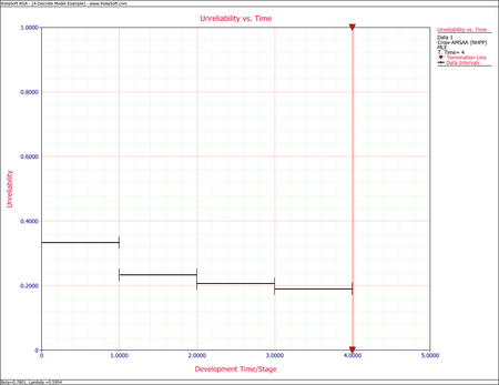


Parameter Estimation for Discrete-Mixed Data
The table below shows the number of failures of each interval of trials and the cumulative number of trials in each interval for a reliability growth test. For example, the first row indicates that for an interval of 14 trials, 5 failures occurred.
| Failures in Interval | Cumulative Trials |
|---|---|
| 5 | 14 |
| 3 | 33 |
| 4 | 48 |
| 0 | 52 |
| 1 | 53 |
| 0 | 57 |
| 1 | 58 |
| 0 | 62 |
| 1 | 63 |
| 0 | 67 |
| 1 | 68 |
Using the RGA software, the parameters of the Crow-AMSAA model are estimated as follows:
- [math]\displaystyle{ \hat{\beta }=0.7950\,\! }[/math]
and:
- [math]\displaystyle{ \hat{\lambda }=0.5588\,\! }[/math]
As we have seen, the Crow-AMSAA instantaneous failure intensity, [math]\displaystyle{ {{\lambda }_{i}}(T)\,\! }[/math], is defined as:
- [math]\displaystyle{ \begin{align} {{\lambda }_{i}}(T)=\lambda \beta {{T}^{\beta -1}},\text{with }T\gt 0,\text{ }\lambda \gt 0\text{ and }\beta \gt 0 \end{align}\,\! }[/math]
Using the parameter estimates, we can calculate the instantaneous unreliability at the end of the test, or [math]\displaystyle{ T=68.\,\! }[/math]
- [math]\displaystyle{ {{R}_{i}}(68)=0.5588\cdot 0.7950\cdot {{68}^{0.7950-1}}=0.1871\,\! }[/math]
This result that can be obtained from the Quick Calculation Pad (QCP), for [math]\displaystyle{ T=68,\,\! }[/math] as seen in the following picture.

The instantaneous reliability can then be calculated as:
- [math]\displaystyle{ \begin{align} {{R}_{inst}}=1-0.1871=0.8129 \end{align}\,\! }[/math]
Failure Times Data Example
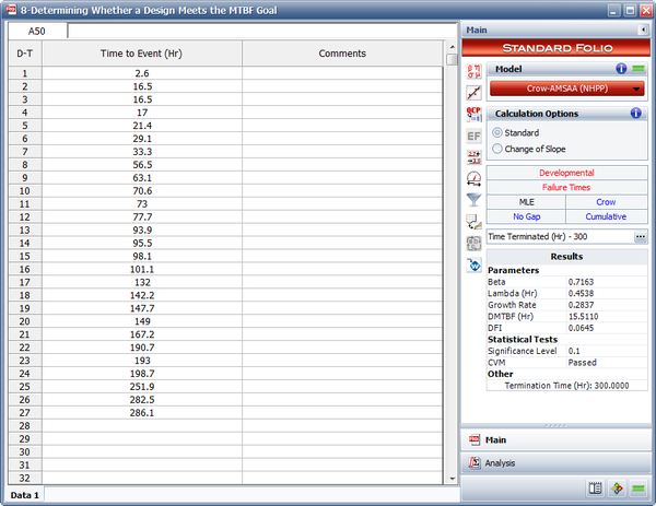
A prototype of a system was tested at the end of one of its design stages. The test was run for a total of 300 hours and 27 failures were observed. The table below shows the collected data set. The prototype has a design specification of an MTBF equal to 10 hours with a 90% confidence level at 300 hours. Do the following:
- Estimate the parameters of the Crow-AMSAA model using maximum likelihood estimation.
- Does the prototype meet the specified goal?
| 2.6 | 56.5 | 98.1 | 190.7 |
| 16.5 | 63.1 | 101.1 | 193 |
| 16.5 | 70.6 | 132 | 198.7 |
| 17 | 73 | 142.2 | 251.9 |
| 21.4 | 77.7 | 147.7 | 282.5 |
| 29.1 | 93.9 | 149 | 286.1 |
| 33.3 | 95.5 | 167.2 |
Solution
- The next figure shows the parameters estimated using RGA.
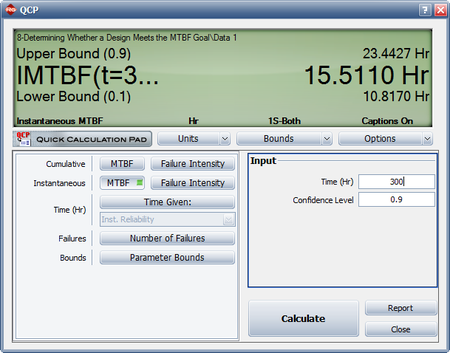
- The instantaneous MTBF with one-sided 90% confidence bounds can be calculated using the Quick Calculation Pad (QCP), as shown next. From the QCP, it is estimated that the lower limit on the MTBF at 300 hours with a 90% confidence level is equal to 10.8170 hours. Therefore, the prototype has met the specified goal.


Failure Times Grouped Data Examples
Example 1
Consider the grouped failure times data given in the following table. Solve for the Crow-AMSAA parameters using MLE.
| Run Number | Cumulative Failures | End Time(hours) | [math]\displaystyle{ \ln{(T_i)}\,\! }[/math] | [math]\displaystyle{ \ln{(T_i)^2}\,\! }[/math] | [math]\displaystyle{ \ln{(\theta_i)}\,\! }[/math] | [math]\displaystyle{ \ln{(T_i)}\cdot\ln{(\theta_i)}\,\! }[/math] |
|---|---|---|---|---|---|---|
| 1 | 2 | 200 | 5.298 | 28.072 | 0.693 | 3.673 |
| 2 | 3 | 400 | 5.991 | 35.898 | 1.099 | 6.582 |
| 3 | 4 | 600 | 6.397 | 40.921 | 1.386 | 8.868 |
| 4 | 11 | 3000 | 8.006 | 64.102 | 2.398 | 19.198 |
| Sum = | 25.693 | 168.992 | 5.576 | 38.321 |
Solution
Using RGA, the value of [math]\displaystyle{ \hat{\beta }\,\! }[/math], which must be solved numerically, is 0.6315. Using this value, the estimator of [math]\displaystyle{ \lambda \,\! }[/math] is:
- [math]\displaystyle{ \begin{align} \hat{\lambda } = & \frac{11}{3,{{000}^{0.6315}}} \\ = & 0.0701 \end{align}\,\! }[/math]
Therefore, the intensity function becomes:
- [math]\displaystyle{ \hat{\rho }(T)=0.0701\cdot 0.6315\cdot {{T}^{-0.3685}}\,\! }[/math]
Example 2
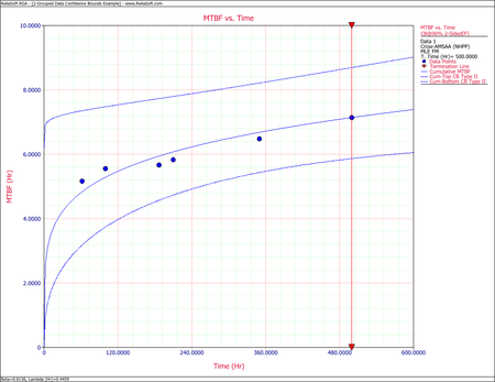
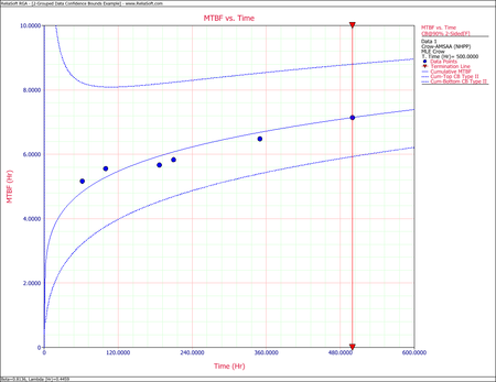
A new helicopter system is under development. System failure data has been collected on five helicopters during the final test phase. The actual failure times cannot be determined since the failures are not discovered until after the helicopters are brought into the maintenance area. However, total flying hours are known when the helicopters are brought in for service, and every 2 weeks each helicopter undergoes a thorough inspection to uncover any failures that may have occurred since the last inspection. Therefore, the cumulative total number of flight hours and the cumulative total number of failures for the 5 helicopters are known for each 2-week period. The total number of flight hours from the test phase is 500, which was accrued over a period of 12 weeks (six 2-week intervals). For each 2-week interval, the total number of flight hours and total number of failures for the 5 helicopters were recorded. The grouped data set is displayed in the following table.
| Interval | Interval Length | Failures in Interval |
|---|---|---|
| 1 | 0 - 62 | 12 |
| 2 | 62 -100 | 6 |
| 3 | 100 - 187 | 15 |
| 4 | 187 - 210 | 3 |
| 5 | 210 - 350 | 18 |
| 6 | 350 - 500 | 16 |
Do the following:
- Estimate the parameters of the Crow-AMSAA model using maximum likelihood estimation.
- Calculate the confidence bounds on the cumulative and instantaneous MTBF using the Fisher Matrix and Crow methods.
Solution
- Using RGA, the value of [math]\displaystyle{ \hat{\beta }\,\! }[/math], must be solved numerically. Once [math]\displaystyle{ \hat{\beta }\,\! }[/math] has been estimated then the value of [math]\displaystyle{ \hat{\lambda }\,\! }[/math] can be determined. The parameter values are displayed below:
- [math]\displaystyle{ \hat{\beta }= 0.81361\,\! }[/math]
- [math]\displaystyle{ \hat{\lambda }= 0.44585\,\! }[/math]
- [math]\displaystyle{ \begin{align} {{\beta }_{L}} = & \hat{\beta }{{e}^{{{z}_{\alpha }}\sqrt{Var(\hat{\beta })}/\hat{\beta }}} \\ = & 0.6546 \\ {{\beta }_{U}} = & \hat{\beta }{{e}^{-{{z}_{\alpha }}\sqrt{Var(\hat{\beta })}/\hat{\beta }}} \\ = & 1.0112 \end{align}\,\! }[/math]
- [math]\displaystyle{ \begin{align} {{\lambda }_{L}} = & \hat{\lambda }{{e}^{{{z}_{\alpha }}\sqrt{Var(\hat{\lambda })}/\hat{\lambda }}} \\ = & 0.14594 \\ {{\lambda }_{U}} = & \hat{\lambda }{{e}^{-{{z}_{\alpha }}\sqrt{Var(\hat{\lambda })}/\hat{\lambda }}} \\ = & 1.36207 \end{align}\,\! }[/math]
- [math]\displaystyle{ \begin{align} {{\beta }_{L}} = & \hat{\beta }(1-S) \\ = & 0.63552 \\ {{\beta }_{U}} = & \hat{\beta }(1+S) \\ = & 0.99170 \end{align}\,\! }[/math]
- [math]\displaystyle{ \begin{align} {{\lambda }_{L}} = & \frac{\chi _{\tfrac{\alpha }{2},2N}^{2}}{2\cdot T_{k}^{\beta }} \\ = & 0.36197 \\ {{\lambda }_{U}} = & \frac{\chi _{1-\tfrac{\alpha }{2},2N+2}^{2}}{2\cdot T_{k}^{\beta }} \\ = & 0.53697 \end{align}\,\! }[/math]
- The Fisher Matrix confidence bounds for the cumulative MTBF and the instantaneous MTBF at the 90% 2-sided confidence level and for [math]\displaystyle{ T=500\,\! }[/math] hour are:
- [math]\displaystyle{ \begin{align} {{[{{m}_{c}}(T)]}_{L}} = & {{{\hat{m}}}_{c}}(t){{e}^{{{z}_{\alpha /2}}\sqrt{Var({{{\hat{m}}}_{c}}(t))}/{{{\hat{m}}}_{c}}(t)}} \\ = & 5.8680 \\ {{[{{m}_{c}}(T)]}_{U}} = & {{{\hat{m}}}_{c}}(t){{e}^{-{{z}_{\alpha /2}}\sqrt{Var({{{\hat{m}}}_{c}}(t))}/{{{\hat{m}}}_{c}}(t)}} \\ = & 8.6947 \end{align}\,\! }[/math]
- [math]\displaystyle{ \begin{align} {{[MTB{{F}_{i}}]}_{L}} = & {{{\hat{m}}}_{i}}(t){{e}^{{{z}_{\alpha /2}}\sqrt{Var({{{\hat{m}}}_{i}}(t))}/{{{\hat{m}}}_{i}}(t)}} \\ = & 6.6483 \\ {{[MTB{{F}_{i}}]}_{U}} = & {{{\hat{m}}}_{i}}(t){{e}^{-{{z}_{\alpha /2}}\sqrt{Var({{{\hat{m}}}_{i}}(t))}/{{{\hat{m}}}_{i}}(t)}} \\ = & 11.5932 \end{align}\,\! }[/math]
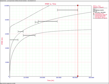
The Crow confidence bounds for the cumulative and instantaneous MTBF at the 90% 2-sided confidence level and for [math]\displaystyle{ T = 500\,\! }[/math]hours are:
- [math]\displaystyle{ \begin{align} {{[{{m}_{c}}(T)]}_{L}} = & \frac{1}{C{{(t)}_{U}}} \\ = & 5.85449 \\ {{[{{m}_{c}}(T)]}_{U}} = & \frac{1}{C{{(t)}_{L}}} \\ = & 8.79822 \end{align}\,\! }[/math]
and:
- [math]\displaystyle{ \begin{align} {{[MTB{{F}_{i}}]}_{L}} = & {{\hat{m}}_{i}}(1-W) \\ = & 6.19623 \\ {{[MTB{{F}_{i}}]}_{U}} = & {{\hat{m}}_{i}}(1+W) \\ = & 11.36223 \end{align}\,\! }[/math]
The next two figures show plots of the Crow confidence bounds for the cumulative and instantaneous MTBF.


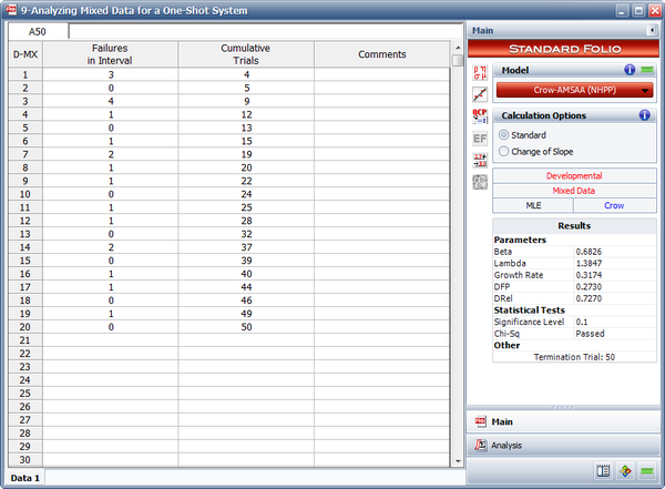
Discrete Mixed Data Example
A one-shot system underwent reliability growth development for a total of 50 trials. The test was performed as a combination of configuration in groups and individual trial by trial. The table below shows the data set obtained from the test. The first column specifies the number of failures that occurred in each interval, and the second column shows the cumulative number of trials in that interval. Do the following:
- Estimate the parameters of the Crow-AMSAA model using maximum likelihood estimators.
- What are the instantaneous reliability and the 2-sided 90% confidence bounds at the end of the test?
- Plot the cumulative reliability with 2-sided 90% confidence bounds.
- If the test was continued for another 25 trials what would the expected number of additional failures be?
| Failures in Interval | Cumulative Trials | Failures in Interval | Cumulative Trials |
|---|---|---|---|
| 3 | 4 | 1 | 25 |
| 0 | 5 | 1 | 28 |
| 4 | 9 | 0 | 32 |
| 1 | 12 | 2 | 37 |
| 0 | 13 | 0 | 39 |
| 1 | 15 | 1 | 40 |
| 2 | 19 | 1 | 44 |
| 1 | 20 | 0 | 46 |
| 1 | 22 | 1 | 49 |
| 0 | 24 | 0 | 50 |
Solution
- The next figure shows the parameters estimated using RGA.
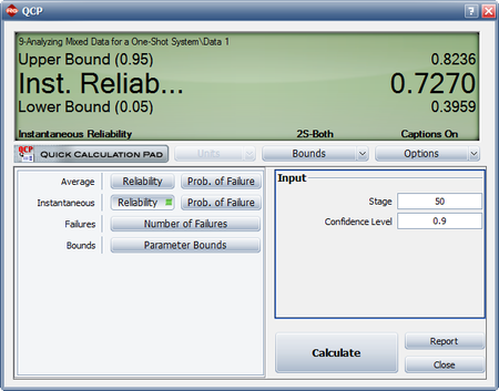
- The figure below shows the calculation of the instantaneous reliability with the 2-sided 90% confidence bounds. From the QCP, it is estimated that the instantaneous reliability at stage 50 (or at the end of the test) is 72.70% with an upper and lower 2-sided 90% confidence bound of 82.36% and 39.59%, respectively.
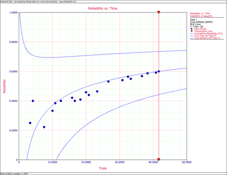
- The following plot shows the cumulative reliability with the 2-sided 90% confidence bounds.
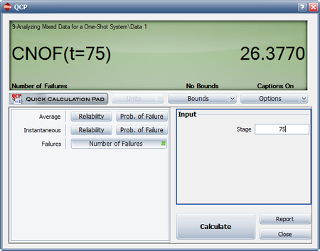
- The last figure shows the calculation of the expected number of failures after 75 trials. From the QCP, it is estimated that the cumulative number of failures after 75 trials is [math]\displaystyle{ 26.3770\approx 27\,\! }[/math]. Since 20 failures occurred in the first 50 trials, the estimated number of additional failures is 7.


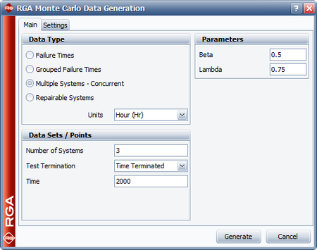
Multiple Systems: Concurrent Operating Times Example
Six systems were subjected to a reliability growth test, and a total of 82 failures were observed. Given the data in the table below, which presents the start/end times and times-to-failure for each system, do the following:
- Estimate the parameters of the Crow-AMSAA model using maximum likelihood estimation.
- Determine how many additional failures would be generated if testing continues until 3,000 hours.
| System # | 1 | 2 | 3 | 4 | 5 | 6 |
| Start Time (Hr) | 0 | 0 | 0 | 0 | 0 | 0 |
| End Time (Hr) | 504 | 541 | 454 | 474 | 436 | 500 |
| Failure Times (Hr) | 21 | 83 | 26 | 36 | 23 | 7 |
| 29 | 83 | 26 | 306 | 46 | 13 | |
| 43 | 83 | 57 | 306 | 127 | 13 | |
| 43 | 169 | 64 | 334 | 166 | 31 | |
| 43 | 213 | 169 | 354 | 169 | 31 | |
| 66 | 299 | 213 | 395 | 213 | 82 | |
| 115 | 375 | 231 | 403 | 213 | 109 | |
| 159 | 431 | 231 | 448 | 255 | 137 | |
| 199 | 231 | 456 | 369 | 166 | ||
| 202 | 231 | 461 | 374 | 200 | ||
| 222 | 304 | 380 | 210 | |||
| 248 | 383 | 415 | 220 | |||
| 248 | 301 | |||||
| 255 | 422 | |||||
| 286 | 437 | |||||
| 286 | 469 | |||||
| 304 | 469 | |||||
| 320 | ||||||
| 348 | ||||||
| 364 | ||||||
| 404 | ||||||
| 410 | ||||||
| 429 |
Solution
- To estimate the parameters [math]\displaystyle{ \hat{\beta }\,\! }[/math] and [math]\displaystyle{ \hat{\lambda}\,\! }[/math], the equivalent single system (ESS) must first be determined. The ESS is given below:
Equivalent Single System Row Time to Event (hr) Row Time to Event (hr) Row Time to Event (hr) Row Time to Event (hr) 1 42 22 498 43 1386 64 2214 2 78 23 654 44 1386 65 2244 3 78 24 690 45 1386 66 2250 4 126 25 762 46 1386 67 2280 5 138 26 822 47 1488 68 2298 6 156 27 954 48 1488 69 2370 7 156 28 996 49 1530 70 2418 8 174 29 996 50 1530 71 2424 9 186 30 1014 51 1716 72 2460 10 186 31 1014 52 1716 73 2490 11 216 32 1014 53 1794 74 2532 12 258 33 1194 54 1806 75 2574 13 258 34 1200 55 1824 76 2586 14 258 35 1212 56 1824 77 2621 15 276 36 1260 57 1836 78 2676 16 342 37 1278 58 1836 79 2714 17 384 38 1278 59 1920 80 2734 18 396 39 1278 60 2004 81 2766 19 492 40 1278 61 2088 82 2766 20 498 41 1320 62 2124 21 498 42 1332 63 2184 Given the ESS data, the value of [math]\displaystyle{ \hat{\beta }\,\! }[/math] is calculated using:
- [math]\displaystyle{ \hat{\beta }=\frac{n}{n\ln {{T}^{*}}-\underset{i=1}{\overset{n}{\mathop{\sum }}}\,\ln {{T}_{i}}}\,\! }[/math]
- [math]\displaystyle{ \hat{\beta }=0.8939\,\! }[/math]
where [math]\displaystyle{ n\,\! }[/math] is the number of failures and [math]\displaystyle{ T^*\,\! }[/math] is the termination time. The termination time is the sum of end times for each of the systems, which equals 2,909.
[math]\displaystyle{ \hat{\lambda}\,\! }[/math] is estimated with:
- [math]\displaystyle{ \hat{\lambda }=\frac{n}{{{T}^{*}}^{\beta }} }[/math]
- [math]\displaystyle{ \hat{\lambda }=0.0657\,\! }[/math]
The next figure shows the parameters estimated using RGA.

- The number of failures can be estimated using the Quick Calculation Pad, as shown next. The estimated number of failures at 3,000 hours is equal to 84.2892 and 82 failures were observed during testing. Therefore, the number of additional failures generated if testing continues until 3,000 hours is equal to [math]\displaystyle{ 84.2892-82=2.2892\approx 3\,\! }[/math]
