Change of Slope Analysis

This article also appears in Reliability growth reference.

The assumption of the Crow-AMSAA (NHPP) model is that the failure intensity is monotonically increasing, decreasing or remaining constant over time. However, there might be cases in which the system design or the operational environment experiences major changes during the observation period and, therefore, a single model will not be appropriate to describe the failure behavior for the entire timeline. RGA incorporates a methodology that can be applied to scenarios where a major change occurs during a reliability growth test. The test data can be broken into two segments with a separate Crow-AMSAA (NHPP) model applied to each segment.

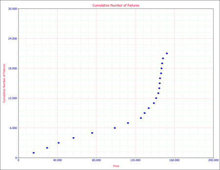
Consider the data in the following plot from a reliability growth test.

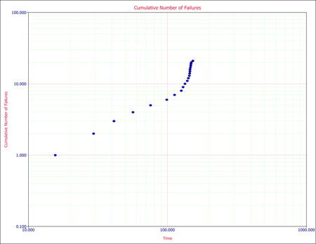
As discussed above, the cumulative number of failures vs. the cumulative time should be linear on logarithmic scales. The next figure shows the data plotted on logarithmic scales.

One can easily recognize that the failure behavior is not constant throughout the duration of the test. Just by observing the data, it can be asserted that a major change occurred at around 140 hours that resulted in a change in the rate of failures. Therefore, using a single model to analyze this data set likely will not be appropriate.

The Change of Slope methodology proposes to split the data into two segments and apply a Crow-AMSAA (NHPP) model to each segment. The time of change that will be used to split the data into the two segments (it will be referred to as [math]\displaystyle{ {{T}_{1}}\,\! }[/math] ) could be estimated just by observing the data, but will most likely be dictated by engineering knowledge of the specific change to the system design or operating conditions. It is important to note that although two separate models will be applied to each segment, the information collected in the first segment (i.e., data up to [math]\displaystyle{ {{T}_{1}}\,\! }[/math] ) will be considered when creating the model for the second segment (i.e., data after [math]\displaystyle{ {{T}_{1}}\,\! }[/math] ). The models presented next can be applied to the reliability growth analysis of a single system or multiple systems.

Model for First Segment (Data up to T₁)

The data up to the point of the change that occurs at [math]\displaystyle{ {{T}_{1}}\,\! }[/math] will be analyzed using the Crow-AMSAA (NHPP) model. Based on the ML equations for [math]\displaystyle{ \lambda \,\! }[/math] and [math]\displaystyle{ \beta \,\! }[/math] (in the section Maximum Likelihood Estimators), the ML estimators of the model are:

[math]\displaystyle{ \widehat{{{\lambda }_{1}}}=\frac{{{n}_{1}}}{T_{1}^{{{\beta }_{1}}}}\,\! }[/math]

and

[math]\displaystyle{ {{\widehat{\beta }}_{1}}=\frac{{{n}_{1}}}{{{n}_{1}}\ln {{T}_{1}}-\underset{i=1}{\overset{{{n}_{1}}}{\mathop{\sum }}}\,\ln {{t}_{i}}}\,\! }[/math]

where:

• [math]\displaystyle{ {{T}_{1}}\,\! }[/math] is the time when the change occurs
• [math]\displaystyle{ {{n}_{1}}\,\! }[/math] is the number of failures observed up to time [math]\displaystyle{ {{T}_{1}}\,\! }[/math]
• [math]\displaystyle{ {{t}_{i}}\,\! }[/math] is the time at which each corresponding failure was observed

The equation for [math]\displaystyle{ \widehat{\beta_{1}}\,\! }[/math] can be rewritten as follows:

[math]\displaystyle{ \begin{align} {{\widehat{\beta }}_{1}}= & \frac{{{n}_{1}}}{{{n}_{1}}\ln {{T}_{1}}-\left( \ln {{t}_{1}}+\ln {{t}_{2}}+...+\ln {{t}_{{{n}_{1}}}} \right)} \\ = & \frac{{{n}_{1}}}{(\ln {{T}_{1}}-\ln {{t}_{1}})+(\ln {{T}_{1}}-\ln {{t}_{2}})+(...)+(\ln {{T}_{1}}-\ln {{t}_{{{n}_{1}}}})} \\ = & \frac{{{n}_{1}}}{\ln \tfrac{{{T}_{1}}}{{{t}_{1}}}+\ln \tfrac{{{T}_{1}}}{{{t}_{2}}}+...+\ln \tfrac{{{T}_{1}}}{{{t}_{{{n}_{1}}}}}} \end{align}\,\! }[/math]

or

[math]\displaystyle{ {{\widehat{\beta }}_{1}}=\frac{{{n}_{1}}}{\underset{i=1}{\overset{{{n}_{1}}}{\mathop{\sum }}}\,\ln \tfrac{{{T}_{1}}}{{{t}_{i}}}}\,\! }[/math]

Model for Second Segment (Data after T₁)

The Crow-AMSAA (NHPP) model will be used again to analyze the data after [math]\displaystyle{ {{T}_{1}}\,\! }[/math]. However, the information collected during the first segment will be used when creating the model for the second segment. Given that, the ML estimators of the model parameters in the second segment are:

[math]\displaystyle{ \widehat{{{\lambda }_{2}}}=\frac{{{n}}}{T_{2}^{{{\beta }_{2}}}}\,\! }[/math]

and:

[math]\displaystyle{ {{\widehat{\beta }}_{2}}=\frac{{{n}_{2}}}{{{n}_{1}}\ln \tfrac{{{T}_{2}}}{{{T}_{1}}}+\underset{i={{n}_{1}}+1}{\overset{n}{\mathop{\sum }}}\,\ln \tfrac{{{T}_{2}}}{{{t}_{i}}}}\,\! }[/math]

where:

• [math]\displaystyle{ {{n}_{2}}\,\! }[/math] is the number of failures that were observed after [math]\displaystyle{ {{T}_{1}}\,\! }[/math]
• [math]\displaystyle{ n={{n}_{1}}+{{n}_{2}}\,\! }[/math] is the total number of failures observed throughout the test
• [math]\displaystyle{ {{T}_{2}}\,\! }[/math] is the end time of the test. The test can either be failure terminated or time terminated

Example - Multiple MLE

The following table gives the failure times obtained from a reliability growth test of a newly designed system. The test has a duration of 660 hours.

Failure Times From a Reliability Growth Test [math]\displaystyle{ \begin{matrix} \text{7}\text{.8} & \text{99}\text{.2} & \text{151} & \text{260}\text{.1} & \text{342} & \text{430}\text{.2} \\ \text{17}\text{.6} & \text{99}\text{.6} & \text{163} & \text{273}\text{.1} & \text{350}\text{.2} & \text{445}\text{.7} \\ \text{25}\text{.3} & \text{100}\text{.3} & \text{174}\text{.5} & \text{274}\text{.7} & \text{355}\text{.2} & \text{475}\text{.9} \\ \text{15} & \text{102}\text{.5} & \text{177}\text{.4} & \text{282}\text{.8} & \text{364}\text{.6} & \text{490}\text{.1} \\ \text{47}\text{.5} & \text{112} & \text{191}\text{.6} & \text{285} & \text{364}\text{.9} & \text{535} \\ \text{54} & \text{112}\text{.2} & \text{192}\text{.7} & \text{315}\text{.4} & \text{366}\text{.3} & \text{580}\text{.3} \\ \text{54}\text{.5} & \text{120}\text{.9} & \text{213} & \text{317}\text{.1} & \text{379}\text{.4} & \text{610}\text{.6} \\ \text{56}\text{.4} & \text{121}\text{.9} & \text{244}\text{.8} & \text{320}\text{.6} & \text{389} & \text{640}\text{.5} \\ \text{63}\text{.6} & \text{125}\text{.5} & \text{249} & \text{324}\text{.5} & \text{394}\text{.9} & {} \\ \text{72}\text{.2} & \text{133}\text{.4} & \text{250}\text{.8} & \text{324}\text{.9} & \text{395}\text{.2} & {} \\ \end{matrix}\,\! }[/math]

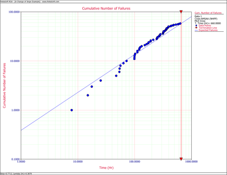
First, apply a single Crow-AMSAA (NHPP) model to all of the data. The following plot shows the expected failures obtained from the model (the line) along with the observed failures (the points).

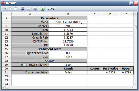
The plot shows that the model does not seem to accurately track the data. This is confirmed by performing the Cramér-von Mises goodness-of-fit test, which checks the hypothesis that the data follows a non-homogeneous Poisson process with a power law failure intensity. The model fails the goodness-of-fit test because the test statistic (0.3309) is higher than the critical value (0.1729) at the 0.1 significance level. The next figure shows a customized report that displays both the calculated parameters and the statistical test results.

Through further investigation, it is discovered that a significant design change occurred at 400 hours of test time. It is suspected that this modification is responsible for the change in the failure behavior.

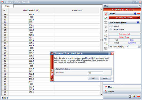
In RGA, you have the option to perform a standard Crow-AMSAA (NHPP) analysis, or perform a Change of Slope analysis where you specify a specific breakpoint, as shown in the following figure. RGA actually creates a grouped data set where the data in Segment 1 is included and defined by a single interval to calculate the Segment 2 parameters. However, these results are equivalent to the parameters estimated using the equations presented here.

Therefore, the Change of Slope methodology is applied to break the data into two segments for analysis. The first segment is set from 0 to 400 hours and the second segment is from 401 to 660 hours (which is the end time of the test). The Crow-AMSAA (NHPP) parameters for the first segment (0-400 hours) are:

[math]\displaystyle{ \widehat{{{\lambda }_{1}}}=\frac{{{n}_{1}}}{T_{1}^{{{\beta }_{1}}}}=\frac{50}{{{400}^{1.0359}}}=0.1008\,\! }[/math]

and

[math]\displaystyle{ {{\widehat{\beta }}_{1}}=\frac{{{n}_{1}}}{\underset{i=1}{\overset{{{n}_{1}}}{\mathop{\sum }}}\,\ln \tfrac{{{T}_{1}}}{{{t}_{i}}}}=\frac{50}{\underset{i=1}{\overset{50}{\mathop{\sum }}}\,\ln \tfrac{400}{{{t}_{i}}}}=1.0359\,\! }[/math]

The Crow-AMSAA (NHPP) parameters for the second segment (401-660 hours) are:

[math]\displaystyle{ \widehat{{{\lambda }_{2}}}=\frac{{{n}}}{T_{2}^{{{\beta }_{2}}}}=\frac{58}{{{660}^{0.2971}}}=8.4304\,\! }[/math]

[math]\displaystyle{ {{\widehat{\beta }}_{2}}=\frac{{{n}_{2}}}{{{n}_{1}}\ln \tfrac{{{T}_{2}}}{{{T}_{1}}}+\underset{i={{n}_{1}}+1}{\overset{n}{\mathop{\sum }}}\,\ln \tfrac{{{T}_{2}}}{{{t}_{i}}}}=\frac{8}{50\ln \tfrac{660}{400}+\underset{i=51}{\overset{58}{\mathop{\sum }}}\,\ln \tfrac{660}{{{T}_{i}}}}=0.2971\,\! }[/math]

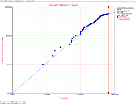
The following figure shows a plot of the two-segment analysis along with the observed data. It is obvious that the Change of Slope method tracks the data more accurately.

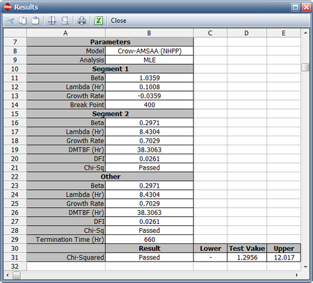
This can also be verified by performing a chi-squared goodness-of-fit test. The chi-squared statistic is 1.2956, which is lower than the critical value of 12.017 at the 0.1 significance level; therefore, the analysis passes the test. The next figure shows a customized report that displays both the calculated parameters and the statistical test results.

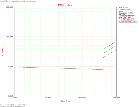
When you have a model that fits the data, it can be used to make accurate predictions and calculations. Metrics such as the demonstrated MTBF at the end of the test or the expected number of failures at later times can be calculated. For example, the following plot shows the instantaneous MTBF vs. time, together with the two-sided 90% confidence bounds. Note that confidence bounds are available for the second segment only. For times up to 400 hours, the parameters of the first segment were used to calculate the MTBF, while the parameters of the second segment were used for times after 400 hours. Also note that the number of failures at the end of segment 1 is not assumed to be equal to the number of failures at the start of segment 2. This can result in a visible jump in the plot, as in this example.

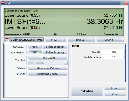
The next figure shows the use of the Quick Calculation Pad (QCP) in the RGA software to calculate the Demonstrated MTBF at the end of the test (instantaneous MTBF at time = 660), together with the two-sided 90% confidence bounds. All the calculations were based on the parameters of the second segment.