Multi-Phase - Mixed Data: Difference between revisions
Kate Racaza (talk | contribs) (Created page with '<noinclude>{{Banner RGA Examples}} ''This example appears in the Reliability Growth and Repairable System Analysis Reference book''. </n…') |
Lisa Hacker (talk | contribs) No edit summary |
||
| (6 intermediate revisions by 2 users not shown) | |||
| Line 1: | Line 1: | ||
<noinclude>{{Banner RGA Examples}} | <noinclude>{{Banner RGA Examples}} | ||
''This example appears in the [ | ''This example appears in the [https://help.reliasoft.com/reference/reliability_growth_and_repairable_system_analysis Reliability growth reference]''. | ||
</noinclude> | </noinclude> | ||
| Line 47: | Line 47: | ||
|F||1||20||BD||5 | |F||1||20||BD||5 | ||
|} | |} | ||
The table also gives the classifications of the failure modes. There are 5 BD modes. Of these 5 modes, 2 are corrected during the test (BD3 and BD4) and 3 have not been corrected by time <math>T=20\,\!</math> (BD1, BD2 and BD5). Do the following: | The table also gives the classifications of the failure modes. There are 5 BD modes. Of these 5 modes, 2 are corrected during the test (BD3 and BD4) and 3 have not been corrected by time <math>T=20\,\!</math> (BD1, BD2 and BD5). Do the following: | ||
#Calculate the parameters of the Crow Extended - Continuous Evaluation model. | |||
#Calculated the demonstrated reliability at the end of the test. | |||
#Calculate parameter <math>p\,\!</math>. | |||
#Calculate the unfixed BD mode failure probability. | |||
#Calculate the nominal growth potential factor. | |||
#Calculate the nominal average effectiveness factor. | |||
#Calculate the discovery failure intensity function at the end of the test. | |||
#Calculate the nominal projected reliability at the end of the test. | |||
#Calculate the nominal growth potential reliability at the end of the test. | |||
'''Solution''' | '''Solution''' | ||
<ol> | |||
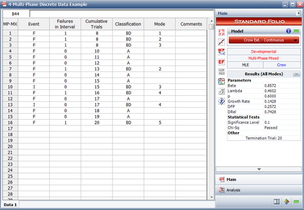
<li>The next figure shows the data entered in the RGA software. | |||
[[File:multi-Phase Discrete Data Entered in RGA.png|600px|center]] | |||
[[File:multi-Phase Discrete Data Entered in RGA.png| | |||
The parameters <math>\beta \,\!</math> and <math>\lambda \,\!</math> are calculated as follows (the calculations for these parameters are presented in detail in the [[Crow- | The parameters <math>\beta \,\!</math> and <math>\lambda \,\!</math> are calculated as follows (the calculations for these parameters are presented in detail in the [[Crow-AMSAA (NHPP)#Parameter_Estimation|Crow-AMSAA (NHPP)]] chapter): | ||
:<math>\widehat{\beta }=0.8572\,\!</math> | |||
and: | |||
:<math>\widehat{\lambda }=0.4602\,\!</math> | |||
</li> | |||
<li>The corresponding demonstrated unreliability is calculated as: | |||
:<math>\begin{align} | |||
{{f}_{D}}=\lambda \beta {{T}^{\beta -1}},\text{with }T>0,\text{ }\lambda >0\text{ and }\beta >0 | {{f}_{D}}=\lambda \beta {{T}^{\beta -1}},\text{with }T>0,\text{ }\lambda >0\text{ and }\beta >0 | ||
\end{align}\,\!</math> | \end{align}\,\!</math> | ||
Using the parameter estimates given above, the instantaneous unreliability at the end of the test (or <math>T=20\,\!</math>) is equal to: | |||
: | :<math>{{f}_{D}}(20)=0.8572\cdot 0.4602\cdot {{20}^{0.8572-1}}=0.2572\,\!</math> | ||
: | The demonstrated reliability is: | ||
:<math>\begin{align} | |||
{{R}_{D}}= & 1-{{f}_{D}} \\ | {{R}_{D}}= & 1-{{f}_{D}} \\ | ||
= & 1-0.2572=0.7428 | = & 1-0.2572=0.7428 | ||
\end{align}\,\!</math> | \end{align}\,\!</math> | ||
Note that in discrete data, we calculate the reliability and not MTBF because we are dealing with the number of trials and not test time. | |||
</li> | |||
<li>Assume that the following effectiveness factors are assigned to the unfixed BD modes: | |||
{|border="1" align="center" style="border-collapse: collapse;" cellpadding="5" cellspacing="5" | {|border="1" align="center" style="border-collapse: collapse;" cellpadding="5" cellspacing="5" | ||
| Line 116: | Line 111: | ||
|} | |} | ||
The parameter <math>p\,\!</math> is the total number of distinct unfixed BD modes at time <math>T\,\!</math> divided by the total number of distinct BD (fixed and unfixed) modes. | |||
: | In this example: | ||
: | :<math>p=\frac{3}{5}=0.6\,\!</math> | ||
</li> | |||
<li>The unfixed BD mode failure probability at time <math>T\,\!</math> is the total number of unfixed BD failures (classified at time <math>T\,\!</math> ) divided by the total trials. Based on the table at the beginning of the example, we have: | |||
:<math>{{f}_{BD, unfixed}}=\frac{4}{20}=0.2\,\!</math> | |||
</li> | |||
<li>The nominal growth potential factor is: | |||
:<math>\begin{align} | |||
{{\lambda }_{NGPFactor}}= & \underset{i=1}{\overset{M}{\mathop \sum }}\,\left( 1-{{d}_{i}} \right)\frac{{{N}_{i}}}{T} \\ | {{\lambda }_{NGPFactor}}= & \underset{i=1}{\overset{M}{\mathop \sum }}\,\left( 1-{{d}_{i}} \right)\frac{{{N}_{i}}}{T} \\ | ||
= & \left( 1-{{d}_{1}} \right)\frac{{{N}_{1}}}{T}+\left( 1-{{d}_{2}} \right)\frac{{{N}_{2}}}{T}+\left( 1-{{d}_{5}} \right)\frac{{{N}_{5}}}{T} \\ | = & \left( 1-{{d}_{1}} \right)\frac{{{N}_{1}}}{T}+\left( 1-{{d}_{2}} \right)\frac{{{N}_{2}}}{T}+\left( 1-{{d}_{5}} \right)\frac{{{N}_{5}}}{T} \\ | ||
| Line 138: | Line 132: | ||
\end{align}\,\!</math> | \end{align}\,\!</math> | ||
</li> | |||
<li>The nominal average effectiveness factor is: | |||
:<math>\begin{align} | |||
{{d}_{N}}= & \frac{\underset{i=1}{\overset{M}{\mathop{\sum }}}\,{{d}_{Ni}}}{M} \\ | {{d}_{N}}= & \frac{\underset{i=1}{\overset{M}{\mathop{\sum }}}\,{{d}_{Ni}}}{M} \\ | ||
= & \frac{0.65+0.70+0.75}{3} \\ | = & \frac{0.65+0.70+0.75}{3} \\ | ||
= & 0.70 | = & 0.70 | ||
\end{align}\,\!</math> | \end{align}\,\!</math> | ||
</li> | |||
<li>The discovery function at time <math>T\,\!</math> is calculated using all the first occurrences of all the BD modes, both fixed and unfixed. In our example, we calculate <math>{{\widehat{\beta }}_{BD}}\,\!</math> and <math>{{\widehat{\lambda }}_{BD}}\,\!</math> using only the unfixed BD modes and excluding the second occurrence of BD2, which results in the following: | |||
:<math>{{\widehat{\beta }}_{BD}}=0.6602\,\!</math> | |||
and: | |||
:<math>{{\widehat{\lambda }}_{BD}}=0.6920\,\!</math> | |||
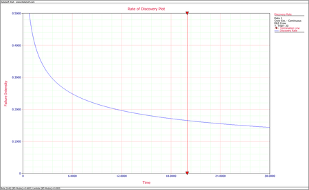
So the discovery failure intensity function at time <math>T=20\,\!</math> is: | |||
:<math>\begin{align} | |||
\widehat{h}(T|BD)= & {{\widehat{\lambda }}_{BD}}{{\widehat{\beta }}_{BD}}{{T}^{{{\widehat{\beta }}_{BD}}-1}} \\ | \widehat{h}(T|BD)= & {{\widehat{\lambda }}_{BD}}{{\widehat{\beta }}_{BD}}{{T}^{{{\widehat{\beta }}_{BD}}-1}} \\ | ||
= & 0.6920\cdot 0.6602\cdot {{20}^{0.6602-1}} \\ | = & 0.6920\cdot 0.6602\cdot {{20}^{0.6602-1}} \\ | ||
| Line 165: | Line 158: | ||
\end{align}\,\!</math> | \end{align}\,\!</math> | ||
The next figure shows the plot for the discovery failure intensity function. | |||
[[Image:rga10.16.png|center|450px]] | |||
[[Image:rga10.16.png|center| | |||
</li> | |||
<li>The nominal projected failure probability at time <math>T=20\,\!</math> is: | |||
:<math>\begin{align} | |||
{{f}_{NP}}= & {{f}_{NGP}}+{{d}_{N}}h(T) \\ | {{f}_{NP}}= & {{f}_{NGP}}+{{d}_{N}}h(T) \\ | ||
= & 0.0701+0.7\cdot 0.16507 \\ | = & 0.0701+0.7\cdot 0.16507 \\ | ||
| Line 179: | Line 171: | ||
\end{align}\,\!</math> | \end{align}\,\!</math> | ||
Therefore, the nominal projected reliability is: | |||
:<math>\begin{align} | |||
{{R}_{P}}= & 1-0.1856= \\ | {{R}_{P}}= & 1-0.1856= \\ | ||
= & 0.8135 | = & 0.8135 | ||
\end{align}\,\!</math> | \end{align}\,\!</math> | ||
</li> | |||
<li>The nominal growth potential unreliability is: | |||
: | :<math>{{f}_{NGP}} = {{f}_{D}} - {{f}_{BD unfixed}} + {{\lambda}_{NGPFactor}} + {{d}_{N}}\cdot p \cdot h(T) - {{d}_{N}}h(T)\,\!</math> | ||
: | Based on the previous calculation for this example, we have: | ||
:<math>\begin{align} | |||
{{f}_{NGP}}= & 0.2572-0.2+0.06+0.7\cdot 0.6\cdot 0.16507-0.7\cdot 0.16507 \\ | {{f}_{NGP}}= & 0.2572-0.2+0.06+0.7\cdot 0.6\cdot 0.16507-0.7\cdot 0.16507 \\ | ||
= & 0.0709 | = & 0.0709 | ||
\end{align}\,\!</math> | \end{align}\,\!</math> | ||
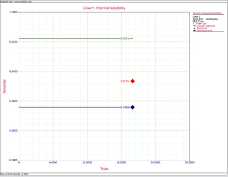
So the nominal growth potential reliability is: | |||
:<math>\begin{align} | |||
{{R}_{NGP}}= & 1-0.0709 \\ | {{R}_{NGP}}= & 1-0.0709 \\ | ||
= & 0.9291 | = & 0.9291 | ||
\end{align}\,\!</math> | \end{align}\,\!</math> | ||
The next figure shows the plot for the instantaneous demonstrated, projected and growth potential reliability. | The next figure shows the plot for the instantaneous demonstrated, projected and growth potential reliability. | ||
[[Image:rga10.17.png|center| | [[Image:rga10.17.png|center|450px]] | ||
</li> | |||
</ol> | |||
Latest revision as of 20:53, 18 September 2023
 |
New format available! This reference is now available in a new format that offers faster page load, improved display for calculations and images and more targeted search.
As of January 2024, this Reliawiki page will not continue to be updated. Please update all links and bookmarks to the latest references at RGA examples and RGA reference examples.
This example appears in the Reliability growth reference.
A one-shot system underwent reliability growth development for a total of 20 trials. The test was performed as a combination of configuration in groups and individual trial-by-trial. The following table shows the obtained data set. The Failures in Interval column specifies the number of failures that occurred in each interval, and the Cumulative Trials column specifies the cumulative number of trials at the end of that interval.
| Mixed Data | ||||
| Event | Failures in Interval | Cumulative Trials | Classification | Mode |
|---|---|---|---|---|
| F | 1 | 8 | BD | 1 |
| F | 1 | 8 | BD | 2 |
| F | 1 | 8 | BD | 3 |
| F | 0 | 10 | A | |
| F | 0 | 11 | A | |
| F | 0 | 12 | A | |
| F | 1 | 13 | BD | 2 |
| F | 0 | 14 | A | |
| F | 0 | 15 | A | |
| I | 0 | 15 | BD | 3 |
| F | 1 | 16 | BD | 4 |
| F | 0 | 17 | A | |
| I | 0 | 17 | BD | 4 |
| F | 0 | 18 | A | |
| F | 0 | 18 | A | |
| F | 1 | 20 | BD | 5 |
The table also gives the classifications of the failure modes. There are 5 BD modes. Of these 5 modes, 2 are corrected during the test (BD3 and BD4) and 3 have not been corrected by time [math]\displaystyle{ T=20\,\! }[/math] (BD1, BD2 and BD5). Do the following:
- Calculate the parameters of the Crow Extended - Continuous Evaluation model.
- Calculated the demonstrated reliability at the end of the test.
- Calculate parameter [math]\displaystyle{ p\,\! }[/math].
- Calculate the unfixed BD mode failure probability.
- Calculate the nominal growth potential factor.
- Calculate the nominal average effectiveness factor.
- Calculate the discovery failure intensity function at the end of the test.
- Calculate the nominal projected reliability at the end of the test.
- Calculate the nominal growth potential reliability at the end of the test.
Solution
- The next figure shows the data entered in the RGA software.
The parameters [math]\displaystyle{ \beta \,\! }[/math] and [math]\displaystyle{ \lambda \,\! }[/math] are calculated as follows (the calculations for these parameters are presented in detail in the Crow-AMSAA (NHPP) chapter):
- [math]\displaystyle{ \widehat{\beta }=0.8572\,\! }[/math]
and:
- [math]\displaystyle{ \widehat{\lambda }=0.4602\,\! }[/math]
- The corresponding demonstrated unreliability is calculated as:
- [math]\displaystyle{ \begin{align} {{f}_{D}}=\lambda \beta {{T}^{\beta -1}},\text{with }T\gt 0,\text{ }\lambda \gt 0\text{ and }\beta \gt 0 \end{align}\,\! }[/math]
- [math]\displaystyle{ {{f}_{D}}(20)=0.8572\cdot 0.4602\cdot {{20}^{0.8572-1}}=0.2572\,\! }[/math]
- [math]\displaystyle{ \begin{align} {{R}_{D}}= & 1-{{f}_{D}} \\ = & 1-0.2572=0.7428 \end{align}\,\! }[/math]
- Assume that the following effectiveness factors are assigned to the unfixed BD modes:
Classification Mode Effectiveness Factor Implemented at End of Phase BD 1 0.65 Phase 1 BD 2 0.70 Phase 1 BD 5 0.75 Phase 1 The parameter [math]\displaystyle{ p\,\! }[/math] is the total number of distinct unfixed BD modes at time [math]\displaystyle{ T\,\! }[/math] divided by the total number of distinct BD (fixed and unfixed) modes.
In this example:
- [math]\displaystyle{ p=\frac{3}{5}=0.6\,\! }[/math]
- The unfixed BD mode failure probability at time [math]\displaystyle{ T\,\! }[/math] is the total number of unfixed BD failures (classified at time [math]\displaystyle{ T\,\! }[/math] ) divided by the total trials. Based on the table at the beginning of the example, we have:
- [math]\displaystyle{ {{f}_{BD, unfixed}}=\frac{4}{20}=0.2\,\! }[/math]
- The nominal growth potential factor is:
- [math]\displaystyle{ \begin{align} {{\lambda }_{NGPFactor}}= & \underset{i=1}{\overset{M}{\mathop \sum }}\,\left( 1-{{d}_{i}} \right)\frac{{{N}_{i}}}{T} \\ = & \left( 1-{{d}_{1}} \right)\frac{{{N}_{1}}}{T}+\left( 1-{{d}_{2}} \right)\frac{{{N}_{2}}}{T}+\left( 1-{{d}_{5}} \right)\frac{{{N}_{5}}}{T} \\ = & \left( 1-0.65 \right)\frac{1}{20}+\left( 1-0.70 \right)\frac{2}{20}+\left( 1-0.75 \right)\frac{1}{20} \\ = & 0.06 \end{align}\,\! }[/math]
- The nominal average effectiveness factor is:
- [math]\displaystyle{ \begin{align} {{d}_{N}}= & \frac{\underset{i=1}{\overset{M}{\mathop{\sum }}}\,{{d}_{Ni}}}{M} \\ = & \frac{0.65+0.70+0.75}{3} \\ = & 0.70 \end{align}\,\! }[/math]
- The discovery function at time [math]\displaystyle{ T\,\! }[/math] is calculated using all the first occurrences of all the BD modes, both fixed and unfixed. In our example, we calculate [math]\displaystyle{ {{\widehat{\beta }}_{BD}}\,\! }[/math] and [math]\displaystyle{ {{\widehat{\lambda }}_{BD}}\,\! }[/math] using only the unfixed BD modes and excluding the second occurrence of BD2, which results in the following:
- [math]\displaystyle{ {{\widehat{\beta }}_{BD}}=0.6602\,\! }[/math]
- [math]\displaystyle{ {{\widehat{\lambda }}_{BD}}=0.6920\,\! }[/math]
- [math]\displaystyle{ \begin{align} \widehat{h}(T|BD)= & {{\widehat{\lambda }}_{BD}}{{\widehat{\beta }}_{BD}}{{T}^{{{\widehat{\beta }}_{BD}}-1}} \\ = & 0.6920\cdot 0.6602\cdot {{20}^{0.6602-1}} \\ = & 0.16507 \end{align}\,\! }[/math]
- The nominal projected failure probability at time [math]\displaystyle{ T=20\,\! }[/math] is:
- [math]\displaystyle{ \begin{align} {{f}_{NP}}= & {{f}_{NGP}}+{{d}_{N}}h(T) \\ = & 0.0701+0.7\cdot 0.16507 \\ = & 0.1865 \end{align}\,\! }[/math]
- [math]\displaystyle{ \begin{align} {{R}_{P}}= & 1-0.1856= \\ = & 0.8135 \end{align}\,\! }[/math]
- The nominal growth potential unreliability is:
- [math]\displaystyle{ {{f}_{NGP}} = {{f}_{D}} - {{f}_{BD unfixed}} + {{\lambda}_{NGPFactor}} + {{d}_{N}}\cdot p \cdot h(T) - {{d}_{N}}h(T)\,\! }[/math]
- [math]\displaystyle{ \begin{align} {{f}_{NGP}}= & 0.2572-0.2+0.06+0.7\cdot 0.6\cdot 0.16507-0.7\cdot 0.16507 \\ = & 0.0709 \end{align}\,\! }[/math]
- [math]\displaystyle{ \begin{align} {{R}_{NGP}}= & 1-0.0709 \\ = & 0.9291 \end{align}\,\! }[/math]