Reliability Importance
 |
This article also appears in the System analysis reference.
Static Reliability Importance
Once the reliability of a system has been determined, engineers are often faced with the task of identifying the least reliable component(s) in the system in order to improve the design. For example, it was observed in RBDs and Analytical System Reliability that the least reliable component in a series system has the biggest effect on the system reliability. In this case, if the reliability of the system is to be improved, then the efforts can best be concentrated on improving the reliability of that component first. In simple systems such as a series system, it is easy to identify the weak components. However, in more complex systems this becomes quite a difficult task. For complex systems, the analyst needs a mathematical approach that will provide the means of identifying and quantifying the importance of each component in the system.
Using reliability importance measures is one method of identifying the relative importance of each component in a system with respect to the overall reliability of the system. The reliability importance, [math]\displaystyle{ {{I}_{R}}\,\! }[/math], of component [math]\displaystyle{ i\,\! }[/math] in a system of [math]\displaystyle{ n\,\! }[/math] components is given by Leemis [17]:
- [math]\displaystyle{ {{I}_{{{R}_{i}}}}=\frac{\partial {{R}_{s}}}{\partial {{R}_{i}}} \ \,\! }[/math]
where:
- [math]\displaystyle{ {{R}_{s}}\,\! }[/math] is the system reliability.
- [math]\displaystyle{ {{R}_{i}}\,\! }[/math] is the component reliability.
- [math]\displaystyle{ {{R}_{s}}\,\! }[/math] is the system reliability.
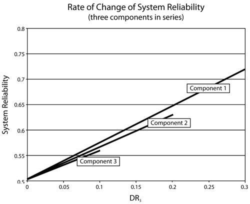
The value of the reliability importance given by equation above depends both on the reliability of a component and its corresponding position in the system. In RBDs and Analytical System Reliability we observed that for a simple series system (three components in series with reliabilities of 0.7, 0.8 and 0.9) the rate of increase of the system reliability was greatest when the least reliable component was improved. In other words, it was observed that Component 1 had the largest reliability importance in the system relative to the other two components (see the figure below). The same conclusion can be drawn by using equation above and obtaining the reliability importance in terms of a value for each component.
Using BlockSim, the reliability importance values for these components can be calculated with the equation above. Using the plot option and selecting the Static Reliability Importance plot type, the following chart can be obtained. Note that the time input required to create this plot is irrelevant for this example because the components are static.
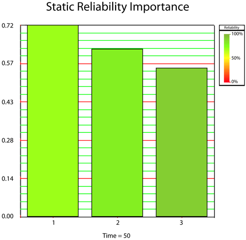
The values shown for each component were obtained using the equation above. The reliability equation for this series system is given by:
- [math]\displaystyle{ {{R}_{_{S}}}={{R}_{1}}\cdot {{R}_{2}}\cdot {{R}_{3}} \ \,\! }[/math]
Taking the partial derivative of the equation above with respect to [math]\displaystyle{ {{R}_{1}}\,\! }[/math] yields:
- [math]\displaystyle{ \begin{align} {{I}_{{{R}_{1}}}}=\frac{\partial {{R}_{s}}}{\partial {{R}_{1}}}= & {{R}_{2}}{{R}_{3}} \\ = & 0.8\cdot 0.9 \\ = & 0.72 \end{align}\,\! }[/math]
Thus the reliability importance of Component 1 is [math]\displaystyle{ {{I}_{{{R}_{1}}}}=\,\! }[/math] 0.72. The reliability importance values for Components 2 and 3 are obtained in a similar manner.
Time-Dependent Reliability Importance
The same concept applies if the components have a time-varying reliability. That is, if [math]\displaystyle{ {{R}_{s}}(t)={{R}_{1}}(t)\cdot {{R}_{2}}(t)\cdot {{R}_{3}}(t)\,\! }[/math], then one could compute [math]\displaystyle{ {{I}_{{{R}_{i}}}}\,\! }[/math] at any time [math]\displaystyle{ x,\,\! }[/math] or [math]\displaystyle{ {{I}_{{{R}_{i}}}}{{(t)}_{_{t=x}}}.\,\! }[/math] This is quantified in the following equation.
- [math]\displaystyle{ {{I}_{{{R}_{i}}}}(t)=\frac{\partial {{R}_{s}}(t)}{\partial {{R}_{i}}(t)}\ \,\! }[/math]
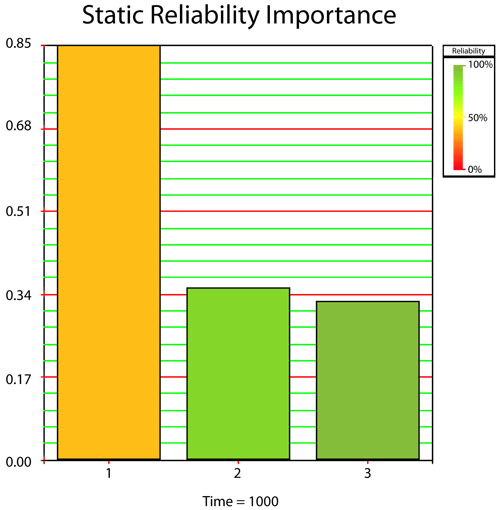
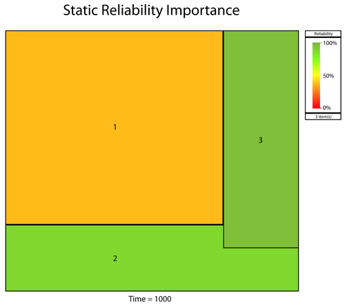
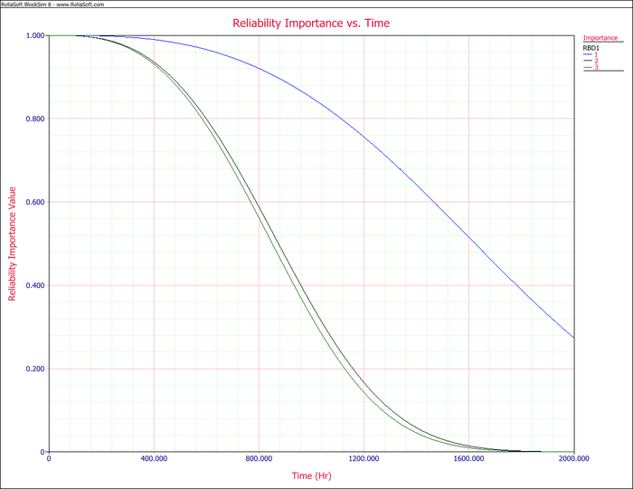
In turn, this can be viewed as either a static plot (at a given time) or as a time-varying plot, as illustrated in the next figures. Specifically, the next three plots present the analysis for three components configured reliability-wise in series following a Weibull distribution with [math]\displaystyle{ \beta =3\,\! }[/math] and [math]\displaystyle{ {{\eta }_{1}}=1,000,\,\! }[/math] [math]\displaystyle{ {{\eta }_{2}}=2,000\,\! }[/math] and [math]\displaystyle{ {{\eta }_{3}}=3,000\,\! }[/math]. The first shows a bar chart of [math]\displaystyle{ {{I}_{{{R}_{i}}}}\,\! }[/math] while the second shows the [math]\displaystyle{ {{I}_{{{R}_{i}}}}\,\! }[/math] in BlockSim's tableau chart format. In this chart, the area of the square is [math]\displaystyle{ {{I}_{{{R}_{i}}}}\,\! }[/math]. Finally, the third plot shows the [math]\displaystyle{ {{I}_{{{R}_{i}}}}(t)\,\! }[/math] vs. time.
Example
Reliability Importance Measures for Failure Modes
Assume that a system has failure modes [math]\displaystyle{ A\,\! }[/math], [math]\displaystyle{ B\,\! }[/math], [math]\displaystyle{ C\,\! }[/math], [math]\displaystyle{ D\,\! }[/math], [math]\displaystyle{ E\,\! }[/math] and [math]\displaystyle{ F\,\! }[/math]. Furthermore, assume that failure of the entire system will occur if:
- Mode [math]\displaystyle{ B\,\! }[/math], [math]\displaystyle{ C\,\! }[/math] or [math]\displaystyle{ F\,\! }[/math] occurs.
- Modes [math]\displaystyle{ A\,\! }[/math] and [math]\displaystyle{ E\,\! }[/math], [math]\displaystyle{ A\,\! }[/math] and [math]\displaystyle{ D\,\! }[/math] or [math]\displaystyle{ E\,\! }[/math] and [math]\displaystyle{ D\,\! }[/math] occur.
- Mode [math]\displaystyle{ B\,\! }[/math], [math]\displaystyle{ C\,\! }[/math] or [math]\displaystyle{ F\,\! }[/math] occurs.
In addition, assume the following failure probabilities for each mode.
- Modes [math]\displaystyle{ A\,\! }[/math] and [math]\displaystyle{ D\,\! }[/math] have a mean time to occurrence of 1,000 hours (i.e., exponential with [math]\displaystyle{ MTTF=1,000).\,\! }[/math]
- Mode [math]\displaystyle{ E\,\! }[/math] has a mean time to occurrence of 100 hours (i.e., exponential with [math]\displaystyle{ MTTF=100).\,\! }[/math]
- Modes [math]\displaystyle{ B\,\! }[/math], [math]\displaystyle{ C\,\! }[/math] and [math]\displaystyle{ F\,\! }[/math] have a mean time to occurrence of 700,000, 1,000,000 and 2,000,000 hours respectively (i.e., exponential with [math]\displaystyle{ MTT{{F}_{B}}=700,000\,\! }[/math], [math]\displaystyle{ MTT{{F}_{C}}=1,000,000\,\! }[/math] and [math]\displaystyle{ MTT{{F}_{F}}=2,000,000).\,\! }[/math]
- Modes [math]\displaystyle{ A\,\! }[/math] and [math]\displaystyle{ D\,\! }[/math] have a mean time to occurrence of 1,000 hours (i.e., exponential with [math]\displaystyle{ MTTF=1,000).\,\! }[/math]
Examine the mode importance for operating times of 100 and 500 hours.
Solution
The RBD for this example is shown next:
The first chart below illustrates [math]\displaystyle{ {{I}_{{{R}_{i}}}}(t=100)\,\! }[/math]. It can be seen that even though [math]\displaystyle{ B\,\! }[/math], [math]\displaystyle{ C\,\! }[/math] and [math]\displaystyle{ F\,\! }[/math] have a much rarer rate of occurrence, they are much more significant at 100 hours. By 500 hours, [math]\displaystyle{ {{I}_{{{R}_{i}}}}(t=500)\,\! }[/math], the effects of the lower reliability components become greatly pronounced and thus they become more important, as can be seen in the second chart. Finally, the behavior of [math]\displaystyle{ {{I}_{{{R}_{i}}}}(t)\,\! }[/math] can be observed in the Reliability Importance vs. Time plot. Note that not all lines are plainly visible in the plot due to overlap.
![Plot of [math]\displaystyle{ {{I}_{{{R}_{i}}}}(t=100)\,\! }[/math] Plot of [math]\displaystyle{ {{I}_{{{R}_{i}}}}(t=100)\,\! }[/math]](/images/9/9b/BS6.6.png)
![Plot of [math]\displaystyle{ {{I}_{{{R}_{i}}}}(t=500)\,\! }[/math] Plot of [math]\displaystyle{ {{I}_{{{R}_{i}}}}(t=500)\,\! }[/math]](/images/thumb/b/bb/6_7.png/600px-6_7.png)
![Plot of [math]\displaystyle{ {{I}_{{{R}_{i}}}}(t)\,\! }[/math] Plot of [math]\displaystyle{ {{I}_{{{R}_{i}}}}(t)\,\! }[/math]](/images/thumb/4/4c/6.8.png/650px-6.8.png)
Importance Measures and FMEA/FMECA
Traditional Failure Mode and Effects Analysis (FMEA/FMECA) relies on Risk Priority Numbers (RPNs) or criticality calculations to identify and prioritize the significance/importance of different failure modes. The RPN methodology (and to some extent, the criticality methodology) tend to be subjective. When conducting these types of analyses, one may wish to incorporate more quantitative metrics, such as the importance measures presented here and/or the RS FCI and RS DECI for repairable systems (which are discussed in later chapters). ReliaSoft's software can be used to export an FMEA/FMECA analysis to BlockSim. The documentation that accompanies Xfmea provides more information on FMEA/FMECA, including both methods of risk assessment.
