Crow Extended Model Examples
 |
New format available! This reference is now available in a new format that offers faster page load, improved display for calculations and images and more targeted search.
As of January 2024, this Reliawiki page will not continue to be updated. Please update all links and bookmarks to the latest references at RGA examples and RGA reference examples.
These examples appear in the Reliability growth reference.
Parameter Estimation
Test-Find-Test Data
Consider the data in the first table below. A system was tested for [math]\displaystyle{ T=400\,\! }[/math] hours. There were a total of [math]\displaystyle{ N=42\,\! }[/math] failures and all corrective actions will be delayed until after the end of the 400 hour test. Each failure has been designated as either an A failure mode (the cause will not receive a corrective action) or a BD mode (the cause will receive a corrective action). There are [math]\displaystyle{ {{N}_{A}}=10\,\! }[/math] A mode failures and [math]\displaystyle{ {{N}_{BD}}=32\,\! }[/math] BD mode failures. In addition, there are [math]\displaystyle{ M=16\,\! }[/math] distinct BD failure modes, which means 16 distinct corrective actions will be incorporated into the system at the end of test. The total number of failures for the [math]\displaystyle{ {{j}^{th}}\,\! }[/math] observed distinct BD mode is denoted by [math]\displaystyle{ {{N}_{j}}\,\! }[/math], and the total number of BD failures during the test is [math]\displaystyle{ {{N}_{BD}}=\underset{j=1}{\overset{M}{\mathop{\sum }}}\,{{N}_{j}}\,\! }[/math]. These values and effectiveness factors are given in the second table
Do the following:
- Determine the projected MTBF and failure intensity.
- Determine the growth potential MTBF and failure intensity.
- Determine the demonstrated MTBF and failure intensity.
| Test-Find-Test Data | ||||||
| [math]\displaystyle{ i\,\! }[/math] | [math]\displaystyle{ {{X}_{i}}\,\! }[/math] | Mode | [math]\displaystyle{ i\,\! }[/math] | [math]\displaystyle{ {{X}_{i}}\,\! }[/math] | Mode | |
|---|---|---|---|---|---|---|
| 1 | 15 | BD1 | 22 | 260.1 | BD1 | |
| 2 | 25.3 | BD2 | 23 | 263.5 | BD8 | |
| 3 | 47.5 | BD3 | 24 | 273.1 | A | |
| 4 | 54 | BD4 | 25 | 274.7 | BD6 | |
| 5 | 56.4 | BD5 | 26 | 285 | BD13 | |
| 6 | 63.6 | A | 27 | 304 | BD9 | |
| 7 | 72.2 | BD5 | 28 | 315.4 | BD4 | |
| 8 | 99.6 | BD6 | 29 | 317.1 | A | |
| 9 | 100.3 | BD7 | 30 | 320.6 | A | |
| 10 | 102.5 | A | 31 | 324.5 | BD12 | |
| 11 | 112 | BD8 | 32 | 324.9 | BD10 | |
| 12 | 120.9 | BD2 | 33 | 342 | BD5 | |
| 13 | 125.5 | BD9 | 34 | 350.2 | BD3 | |
| 14 | 133.4 | BD10 | 35 | 364.6 | BD10 | |
| 15 | 164.7 | BD9 | 36 | 364.9 | A | |
| 16 | 177.4 | BD10 | 37 | 366.3 | BD2 | |
| 17 | 192.7 | BD11 | 38 | 373 | BD8 | |
| 18 | 213 | A | 39 | 379.4 | BD14 | |
| 19 | 244.8 | A | 40 | 389 | BD15 | |
| 20 | 249 | BD12 | 41 | 394.9 | A | |
| 21 | 250.8 | A | 42 | 395.2 | BD16 | |
| Effectiveness Factors for the Unique BD Modes | |||
| BD Mode | Number [math]\displaystyle{ {{N}_{j}}\,\! }[/math] | First Occurrence | EF [math]\displaystyle{ {{d}_{i}}\,\! }[/math] |
|---|---|---|---|
| 1 | 2 | 15.0 | .67 |
| 2 | 3 | 25.3 | .72 |
| 3 | 2 | 47.5 | .77 |
| 4 | 2 | 54.0 | .77 |
| 5 | 3 | 54.0 | .87 |
| 6 | 2 | 99.6 | .92 |
| 7 | 1 | 100.3 | .50 |
| 8 | 3 | 112.0 | .85 |
| 9 | 3 | 125.5 | .89 |
| 10 | 4 | 133.4 | .74 |
| 11 | 1 | 192.7 | .70 |
| 12 | 2 | 249.0 | .63 |
| 13 | 1 | 285.0 | .64 |
| 14 | 1 | 379.4 | .72 |
| 15 | 1 | 389.0 | .69 |
| 16 | 1 | 395.2 | .46 |
Solution
- The maximum likelihood estimates of [math]\displaystyle{ {{\beta }_{BD}}\,\! }[/math] and [math]\displaystyle{ {{\lambda }_{BD}}\,\! }[/math] are determined to be:
- [math]\displaystyle{ \begin{align} {{{\hat{\beta }}}_{BD}} = & \frac{M}{\underset{i=1}{\overset{M}{\mathop{\sum }}}\,\ln (\tfrac{T}{{{X}_{i}}})} \\ = & 0.7970 \\ {{{\hat{\lambda }}}_{BD}} = & 0.1350 \end{align}\,\! }[/math]
- [math]\displaystyle{ \begin{align} {{\overline{\beta }}_{BD}} = & \frac{M-1}{M}{{{\hat{\beta }}}_{BD}} \\ = & 0.7472 \end{align}\,\! }[/math]
- [math]\displaystyle{ \begin{align} r(T) = & \left( \frac{{{N}_{A}}}{T}+\underset{i=1}{\overset{M}{\mathop \sum }}\,(1-{{d}_{i}})\frac{{{N}_{i}}}{T} \right)+\overline{d}\left( \frac{M}{T}{{\overline{\beta }}_{BD}} \right) \\ = & 0.0661 \end{align}\,\! }[/math]
- [math]\displaystyle{ M\widehat{T}B{{F}_{P}}={{[r(T)]}^{-1}}=15.127\,\! }[/math]
- To estimate the maximum reliability that can be attained with this management strategy, use the following calculations.
- [math]\displaystyle{ \begin{align} {{N}_{A}}/T=0.0250 \end{align}\,\! }[/math]
- [math]\displaystyle{ \frac{1}{T}\underset{i=1}{\overset{16}{\mathop \sum }}\,(1-{{d}_{i}}){{N}_{i}}=0.0196\,\! }[/math]
- [math]\displaystyle{ \begin{align} {{\widehat{r}}_{GP}}(T) = & \left( \frac{{{N}_{A}}}{T}+\underset{i=1}{\overset{M}{\mathop \sum }}\,(1-{{d}_{i}})\frac{{{N}_{i}}}{T} \right) \\ = & 0.0250+0.0196 \\ = & 0.0446 \end{align}\,\! }[/math]
- [math]\displaystyle{ M\widehat{T}B{{F}_{GP}}={{[{{\widehat{r}}_{GP}}]}^{-1}}=22.4467\,\! }[/math]
- The demonstrated failure intensity and MTBF are estimated by:
- [math]\displaystyle{ \begin{align} {{\widehat{\lambda }}_{D}}(T) = & \frac{{{N}_{A}}+{{N}_{BD}}}{T} \\ = & \frac{42}{400} \\ = & 0.1050 \end{align}\,\! }[/math]
- [math]\displaystyle{ \begin{align} M\widehat{T}B{{F}_{D}} = & {{[{{\widehat{\lambda }}_{D}}(T)]}^{-1}} \\ = & 9.5238 \end{align}\,\! }[/math]


Confidence Bounds
Calculate the 2-sided 90% confidence bounds on the demonstrated, projected and growth potential failure intensity for the Test-Find-Test data given above.
Solution
The estimated demonstrated failure intensity is [math]\displaystyle{ {{\widehat{\lambda }}_{D}}(T)=\tfrac{{{N}_{A}}+{{N}_{B}}}{T}=0.1050\,\! }[/math]. Based on this value, the Fisher Matrix confidence bounds for the demonstrated failure intensity at the 90% confidence level are:
- [math]\displaystyle{ \begin{align} {{[{{\lambda }_{D}}(T)]}_{L}} = & {{{\hat{\lambda }}}_{D}}(T)+\frac{{{C}^{2}}}{2}-\sqrt{{{{\hat{\lambda }}}_{D}}(T){{C}^{2}}+\frac{{{C}^{4}}}{4}} \\ = & 0.08152 \end{align}\,\! }[/math]
- [math]\displaystyle{ \begin{align} {{[{{\lambda }_{D}}(T)]}_{U}} = & {{{\hat{\lambda }}}_{D}}(T)+\frac{{{C}^{2}}}{2}+\sqrt{{{{\hat{\lambda }}}_{D}}(T){{C}^{2}}+\frac{{{C}^{4}}}{4}} \\ = & 0.13525 \end{align}\,\! }[/math]
The Crow confidence bounds for the demonstrated failure intensity at the 90% confidence level are:
- [math]\displaystyle{ \begin{align} {{[{{\lambda }_{D}}(T)]}_{L}} = & {{\widehat{\lambda }}_{D}}(T)\frac{\chi _{(2N,1-\alpha /2)}^{2}}{2N} \\ = & 0.07985 \\ {{[{{\lambda }_{D}}(T)]}_{U}} = & {{\widehat{\lambda }}_{D}}(T)\frac{\chi _{(2N,\alpha /2)}^{2}}{2N} \\ = & 0.13299 \end{align}\,\! }[/math]
The projected failure intensity is:
- [math]\displaystyle{ \begin{align} \hat{\lambda_{p}} &= \frac{N_{i}}{T}+\sum_{i=1}^{M}(1-d_{i})\frac{N}{T}+\overline{d}\left(\frac{M}{T}\overline{\beta} \right )\\ &= 0.06611 \end{align} }[/math]
Based on this value, the Fisher Matrix confidence bounds at the 90% confidence level for the projected failure intensity are:
- [math]\displaystyle{ \begin{align} {{[{{{\hat{\lambda }}}_{P}}(T)]}_{L}} = & {{{\hat{\lambda }}}_{P}}(T){{e}^{{{z}_{\alpha }}\sqrt{Var({{{\hat{\lambda }}}_{P}}(T))}/{{{\hat{\lambda }}}_{P}}(T)}} \\ = & 0.04902 \end{align}\,\! }[/math]
- [math]\displaystyle{ \begin{align} {{[{{{\hat{\lambda }}}_{P}}(T)]}_{U}} = & {{{\hat{\lambda }}}_{P}}(T){{e}^{-{{z}_{\alpha }}\sqrt{Var({{{\hat{\lambda }}}_{P}}(T))}/{{{\hat{\lambda }}}_{P}}(T)}} \\ = & 0.08915 \end{align}\,\! }[/math]
The Crow confidence bounds for the projected failure intensity are:
- [math]\displaystyle{ \begin{align} {{[{{\lambda }_{P}}(T)]}_{L}} = & {{{\hat{\lambda }}}_{P}}(T)+\frac{{{C}^{2}}}{2}-\sqrt{{{{\hat{\lambda }}}_{P}}(T)\cdot {{C}^{2}}+\frac{{{C}^{4}}}{4}} \\ = & 0.04807 \\ {{[{{\lambda }_{P}}(T)]}_{U}} = & {{{\hat{\lambda }}}_{P}}(T)+\frac{{{C}^{2}}}{2}+\sqrt{{{{\hat{\lambda }}}_{P}}(T)\cdot \ \,{{C}^{2}}+\frac{{{C}^{4}}}{4}} \\ = & 0.09090 \end{align}\,\! }[/math]
The growth potential failure intensity is:
- [math]\displaystyle{ \widehat{r}_{GP} (T) = \left (\frac{N_A}{T} + \sum_{i=1}^M (1-d_i) \tfrac{N_i}{T} \right ) = 0.04455 \,\! }[/math].
Based on this value, the Fisher Matrix and Crow confidence bounds at the 90% confidence level for the growth potential failure intensity are:
- [math]\displaystyle{ \begin{align} {{r}_{L}} = & {{{\hat{r}}}_{GP}}+\frac{{{C}^{2}}}{2}-\sqrt{{{{\hat{r}}}_{GP}}{{C}^{2}}+\frac{{{C}^{4}}}{4}} \\ = & 0.03020 \\ {{r}_{U}} = & {{{\hat{r}}}_{GP}}+\frac{{{C}^{2}}}{2}+\sqrt{{{{\hat{r}}}_{GP}}{{C}^{2}}+\frac{{{C}^{4}}}{4}} \\ = & 0.0656 \end{align}\,\! }[/math]
The figure below shows the Fisher Matrix confidence bounds at the 90% confidence level for the demonstrated, projected and growth potential failure intensity.

The following figure shows these bounds based on the Crow method.

Test-Fix-Find-Test Data
Consider the data given in the first table below. There were 56 total failures and [math]\displaystyle{ T=400\,\! }[/math]. The effectiveness factors of the unique BD modes are given in the second table. Determine the following:
- Calculate the demonstrated MTBF and failure intensity.
- Calculate the projected MTBF and failure intensity.
- What is the rate at which unique BD modes are being generated during this test?
- If the test continues for an additional 50 hours, what is the minimum number of new unique BD modes expected to be generated?
| Test-Fix-Find-Test Data | |||||
| [math]\displaystyle{ i\,\! }[/math] | [math]\displaystyle{ {{X}_{i}}\,\! }[/math] | Mode | [math]\displaystyle{ i\,\! }[/math] | [math]\displaystyle{ {{X}_{i}}\,\! }[/math] | Mode |
|---|---|---|---|---|---|
| 1 | 0.7 | BC17 | 29 | 192.7 | BD11 |
| 2 | 3.7 | BC17 | 30 | 213 | A |
| 3 | 13.2 | BC17 | 31 | 244.8 | A |
| 4 | 15 | BD1 | 32 | 249 | BD12 |
| 5 | 17.6 | BC18 | 33 | 250.8 | A |
| 6 | 25.3 | BD2 | 34 | 260.1 | BD1 |
| 7 | 47.5 | BD3 | 35 | 263.5 | BD8 |
| 8 | 54 | BD4 | 36 | 273.1 | A |
| 9 | 54.5 | BC19 | 37 | 274.7 | BD6 |
| 10 | 56.4 | BD5 | 38 | 282.8 | BC27 |
| 11 | 63.6 | A | 39 | 285 | BD13 |
| 12 | 72.2 | BD5 | 40 | 304 | BD9 |
| 13 | 99.2 | BC20 | 41 | 315.4 | BD4 |
| 14 | 99.6 | BD6 | 42 | 317.1 | A |
| 15 | 100.3 | BD7 | 43 | 320.6 | A |
| 16 | 102.5 | A | 44 | 324.5 | BD12 |
| 17 | 112 | BD8 | 45 | 324.9 | BD10 |
| 18 | 112.2 | BC21 | 46 | 342 | BD5 |
| 19 | 120.9 | BD2 | 47 | 350.2 | BD3 |
| 20 | 121.9 | BC22 | 48 | 355.2 | BC28 |
| 21 | 125.5 | BD9 | 49 | 364.6 | BD10 |
| 22 | 133.4 | BD10 | 50 | 364.9 | A |
| 23 | 151 | BC23 | 51 | 366.3 | BD2 |
| 24 | 163 | BC24 | 52 | 373 | BD8 |
| 25 | 164.7 | BD9 | 53 | 379.4 | BD14 |
| 26 | 174.5 | BC25 | 54 | 389 | BD15 |
| 27 | 177.4 | BD10 | 55 | 394.9 | A |
| 28 | 191.6 | BC26 | 56 | 395.2 | BD16 |
| Effectiveness Factors for the Unique BD Modes | |
| BD Mode | EF [math]\displaystyle{ {{d}_{i}}\,\! }[/math] |
|---|---|
| 1 | .67 |
| 2 | .72 |
| 3 | .77 |
| 4 | .77 |
| 5 | .87 |
| 6 | .92 |
| 7 | .50 |
| 8 | .85 |
| 9 | .89 |
| 10 | .74 |
| 11 | .70 |
| 12 | .63 |
| 13 | .64 |
| 14 | .72 |
| 15 | .69 |
| 16 | .46 |
Solution
- In order to obtain [math]\displaystyle{ {{\widehat{\lambda }}_{CA}}\,\! }[/math], use the traditional Crow-AMSAA model for test-fix-test to fit all 56 data points, regardless of the failure mode classification to get:
- [math]\displaystyle{ \begin{align} \widehat{\beta }= & 0.91026 \\ \widehat{\lambda }= & 0.23969 \end{align}\,\! }[/math]
- [math]\displaystyle{ \begin{align} {{\widehat{\lambda }}_{CA}} = & \widehat{\lambda }\widehat{\beta }{{T}^{\widehat{\beta }-1}} \\ = & 0.23969\times 0.91026\times {{400}^{(0.91026-1)}} \\ = & 0.12744 \end{align}\,\! }[/math]
- [math]\displaystyle{ {{\widehat{M}}_{CA}}={{[{{\widehat{\lambda }}_{CA}}]}^{-1}}=7.84708\,\! }[/math]
- For this data set, [math]\displaystyle{ M=16\,\! }[/math] and [math]\displaystyle{ T=400\,\! }[/math].
- [math]\displaystyle{ {{\widehat{\lambda }}_{BD}}=\frac{{{N}_{BD}}}{T}=\frac{32}{400}=0.08\,\! }[/math]
- [math]\displaystyle{ \overline{d}=\underset{i=1}{\overset{M}{\mathop \sum }}\,{{d}_{i}}/M=0.72125\,\! }[/math]
- [math]\displaystyle{ \underset{i=1}{\overset{16}{\mathop \sum }}\,(1-{{d}_{i}}){{N}_{i}}/T=0.01955\,\! }[/math]
- [math]\displaystyle{ \begin{align} {{{\hat{\beta }}}_{BD}}= & 0.74715 \\ {{{\hat{\lambda }}}_{BD}} = & 0.18197 \end{align}\,\! }[/math]
- [math]\displaystyle{ \overline{d}\widehat{h}(T|BD)=0.0215\,\! }[/math]
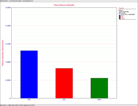
- [math]\displaystyle{ \begin{align} {{\widehat{\lambda }}_{EM}} = & {{\widehat{\lambda }}_{CA}}-{{\widehat{\lambda }}_{BD}}+\underset{i=1}{\overset{K}{\mathop \sum }}\,(1-{{d}_{i}})\frac{{{N}_{i}}}{T}+\overline{d}\widehat{h}(T|BD) \\ = & 0.12744-0.08+0.0196+0.0215 \\ = & 0.08854 \end{align}\,\! }[/math]
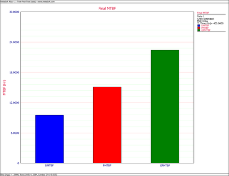
- [math]\displaystyle{ \begin{align} {{\widehat{M}}_{EM}} = & {{[{{\widehat{\lambda }}_{EM}}]}^{-1}} \\ = & 11.29418 \end{align}\,\! }[/math]
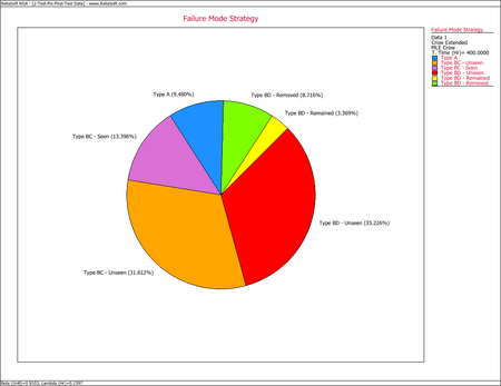
This pie chart shows that 9.48% of the system's failure intensity has been left in (A modes), 31.81% of the failure intensity due to the BC modes has not been seen yet and 13.40% was removed during the test (BC modes - seen). In addition, 33.23% of the failure intensity due to the BD modes has not been seen yet, 3.37% will remain in the system since the corrective actions will not be completely effective at eliminating the identified failure modes, and 8.72% will be removed after the delayed corrective actions.
- The rate at which unique BD modes are being generated is equal to [math]\displaystyle{ h{{(T|BD)}^{-1}}\,\! }[/math], where:
- [math]\displaystyle{ \begin{align} h{{(T|BD)}^{-1}} = & \frac{1}{{{\widehat{\lambda }}_{BD}}{{\widehat{\beta }}_{BD}}{{T}^{{{\widehat{\beta }}_{BD}}-1}}} \\ = & \frac{T}{M{{\widehat{\beta }}_{BD}}} \\ = & 33.4605 \end{align}\,\! }[/math]
- Unique BD modes are being generated every 33.4605 hours. If the test continues for another 50 hours, then at least one new unique BD mode would be expected to be seen from this additional testing.
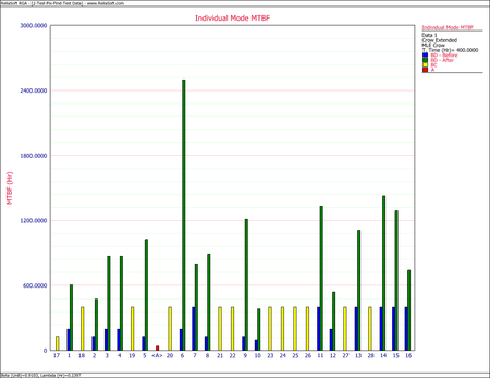
As shown in the next figure, the MTBF of each individual failure mode can be plotted, and the failure modes with the lowest MTBF can be identified. These are the failure modes that cause the majority of the system failures.


Confidence Bounds
Calculate the 2-sided confidence bounds at the 90% confidence level on the demonstrated, projected and growth potential MTBF for the Test-Fix-Find-Test data given above.
Solution
For this example, there are A, BC and BD failure modes, so the estimated demonstrated failure intensity, [math]\displaystyle{ {{\hat{\lambda }}_{D}}(T)\,\! }[/math], is simply the Crow-AMSAA model applied to all A, BC, and BD data.
- [math]\displaystyle{ {{\hat{\lambda }}_{D}}(T)={{\widehat{\lambda }}_{CA}}=\widehat{\lambda }\widehat{\beta }{{T}^{\widehat{\beta }-1}}=0.12744\,\! }[/math]
Therefore, the demonstrated MTBF is:
- [math]\displaystyle{ MTB{{F}_{D}}={{[{{\hat{\lambda }}_{D}}(T)]}^{-1}}=7.84708\,\! }[/math]
Based on this value, the Fisher Matrix confidence bounds for the demonstrated failure intensity at the 90% confidence level are:
- [math]\displaystyle{ \begin{align} {{[{{\lambda }_{D}}(T)]}_{L}} = & {{{\hat{\lambda }}}_{CA}}(T){{e}^{{{z}_{\alpha }}\sqrt{Var({{{\hat{\lambda }}}_{CA}}(T))}/{{{\hat{\lambda }}}_{CA}}(T)}} \\ = & 0.09339 \end{align}\,\! }[/math]
- [math]\displaystyle{ \begin{align} {{[{{\lambda }_{D}}(T)]}_{U}} = & {{{\hat{\lambda }}}_{CA}}(T){{e}^{-{{z}_{\alpha }}\sqrt{Var({{{\hat{\lambda }}}_{CA}}(T))}/{{{\hat{\lambda }}}_{CA}}(T)}} \\ = & 0.17390 \end{align}\,\! }[/math]
The Fisher Matrix confidence bounds for the demonstrated MTBF at the 90% confidence level are:
- [math]\displaystyle{ \begin{align} MTB{{F}_{{{D}_{L}}}} = & \frac{1}{{{[{{\lambda }_{D}}(T)]}_{U}}} \\ = & 5.75054 \\ MTB{{F}_{{{D}_{U}}}} = & \frac{1}{{{[{{\lambda }_{D}}(T)]}_{L}}} \\ = & 10.70799 \end{align}\,\! }[/math]
The Crow confidence bounds for the demonstrated MTBF at the 90% confidence level are:
- [math]\displaystyle{ \begin{align} MTB{{F}_{{{D}_{L}}}} = & \frac{1}{{{[{{\lambda }_{D}}(T)]}_{U}}} \\ = & \frac{1}{{{\widehat{\lambda }}_{D}}(T)\tfrac{{{\chi }^{2}}(2N,\alpha /2)}{2N}} \\ = & 5.6325 \\ MTB{{F}_{{{D}_{U}}}} = & \frac{1}{{{[{{\lambda }_{D}}(T)]}_{L}}} \\ = & \frac{1}{{{\widehat{\lambda }}_{D}}(T)\tfrac{{{\chi }^{2}}(2N,1-\alpha /2)}{2N}} \\ = & 10.8779 \end{align}\,\! }[/math]
The projected failure intensity is:
- [math]\displaystyle{ \begin{align} \hat{\lambda}_P (T) &= \widehat{\lambda}_{CA} - \widehat{\lambda}_{BD} + \sum_{i=1}^M (1-d_i) \tfrac{N_i}{T} + \bar{d}\widehat{h}(T|BD) \\ &= 0.0885 \,\! \end{align} }[/math]
Based on this value, the Fisher Matrix confidence bounds at the 90% confidence level for the projected failure intensity are:
- [math]\displaystyle{ \begin{align} {{[{{\lambda }_{P}}(T)]}_{L}} = & {{{\hat{\lambda }}}_{P}}(T){{e}^{{{z}_{\alpha }}\sqrt{Var({{{\hat{\lambda }}}_{P}}(T))}/{{{\hat{\lambda }}}_{P}}(T)}} \\ = & 0.0681 \end{align}\,\! }[/math]
- [math]\displaystyle{ \begin{align} {{[{{\lambda }_{P}}(T)]}_{U}} = & {{{\hat{\lambda }}}_{P}}(T){{e}^{-{{z}_{\alpha }}\sqrt{Var({{{\hat{\lambda }}}_{P}}(T))}/{{{\hat{\lambda }}}_{P}}(T)}} \\ = & 0.1152 \end{align}\,\! }[/math]
The Fisher Matrix confidence bounds for the projected MTBF at the 90% confidence level are:
- [math]\displaystyle{ \begin{align} MTB{{F}_{{{P}_{L}}}} = & \frac{1}{{{[{{\lambda }_{P}}(T)]}_{U}}} \\ = & 8.6818 \\ MTB{{F}_{{{P}_{U}}}} = & \frac{1}{{{[{{\lambda }_{P}}(T)]}_{L}}} \\ = & 14.6926 \end{align}\,\! }[/math]
The Crow confidence bounds for the projected failure intensity are:
- [math]\displaystyle{ \begin{align} {{[{{\lambda }_{P}}(T)]}_{L}} = & {{{\hat{\lambda }}}_{P}}(T)+\frac{{{C}^{2}}}{2}-\sqrt{{{{\hat{\lambda }}}_{P}}(T)\cdot \ \,{{C}^{2}}+\frac{{{C}^{4}}}{4}} \\ = & 0.0672 \\ {{[{{\lambda }_{P}}(T)]}_{U}} = & {{{\hat{\lambda }}}_{P}}(T)+\frac{{{C}^{2}}}{2}+\sqrt{{{{\hat{\lambda }}}_{P}}(T)\cdot {{C}^{2}}+\frac{{{C}^{4}}}{4}} \\ = & 0.1166 \end{align}\,\! }[/math]
The Crow confidence bounds for the projected MTBF at the 90% confidence level are:
- [math]\displaystyle{ \begin{align} MTB{{F}_{{{P}_{L}}}} = & \frac{1}{{{[{{\widehat{\lambda }}_{P}}(T)]}_{U}}} \\ = & 8.5743 \\ MTB{{F}_{{{P}_{U}}}} = & \frac{1}{{{[{{\widehat{\lambda }}_{P}}(T)]}_{L}}} \\ = & 14.8769 \end{align}\,\! }[/math]
The growth potential failure intensity is:
- [math]\displaystyle{ \widehat{\lambda}_{GP} = \widehat{\lambda}_{CA} - \widehat{\lambda}_{BD} + \sum_{i=1}^M (1-d_i) \tfrac{N_i}{T} = 0.0670 \,\! }[/math]
Based on this value, the Fisher Matrix and Crow confidence bounds at the 90% confidence level for the growth potential failure intensity are:
- [math]\displaystyle{ \begin{align} {{r}_{L}} = & {{{\hat{r}}}_{GP}}+\frac{{{C}^{2}}}{2}-\sqrt{{{{\hat{r}}}_{GP}}{{C}^{2}}+\frac{{{C}^{4}}}{4}} \\ = & 0.0488 \\ {{r}_{U}} = & {{{\hat{r}}}_{GP}}+\frac{{{C}^{2}}}{2}+\sqrt{{{{\hat{r}}}_{GP}}{{C}^{2}}+\frac{{{C}^{4}}}{4}} \\ = & 0.0919 \end{align}\,\! }[/math]
The Fisher Matrix and Crow confidence bounds for the growth potential MTBF at the 90% confidence level are:
- [math]\displaystyle{ \begin{align} MTB{{F}_{G{{P}_{L}}}} = & \frac{1}{{{r}_{U}}} \\ = & 10.8790 \\ MTB{{F}_{G{{P}_{U}}}} = & \frac{1}{{{r}_{L}}} \\ = & 20.4855 \end{align}\,\! }[/math]
The figure below shows the Fisher Matrix confidence bounds at the 90% confidence level for the demonstrated, projected and growth potential MTBF.

The next figure shows these bounds based on the Crow method.

Grouped Failure Times Data Example
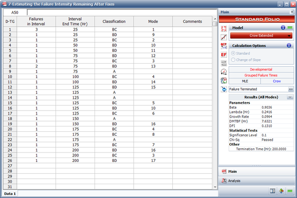
A reliability growth test was conducted for 200 hours. Some of the corrective actions were applied during the test while others were delayed until after the test was completed. The tables below give the data set and the effectiveness factors for the BD modes. Do the following:
- Estimate the parameters of the Crow Extended model.
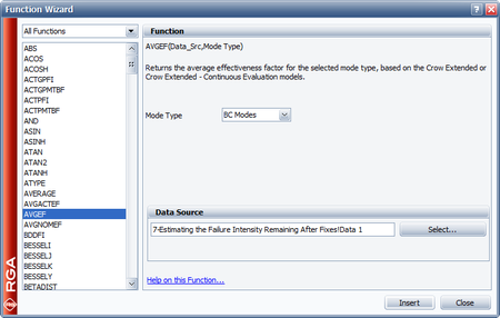
- Determine the average effectiveness factor of the BC modes using the Function Wizard.
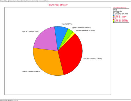
- What percent of the failure intensity will be left in the system due to the BD modes after implementing the delayed fixes?
| Grouped Failure Times Data | |||
| Number at Event | Time to Event | Classification | Mode |
|---|---|---|---|
| 3 | 25 | BC | 1 |
| 1 | 25 | BD | 9 |
| 1 | 25 | BC | 2 |
| 1 | 50 | BD | 10 |
| 1 | 50 | BD | 11 |
| 1 | 75 | BD | 12 |
| 1 | 75 | BC | 3 |
| 2 | 75 | BD | 13 |
| 1 | 75 | A | |
| 1 | 100 | BC | 4 |
| 1 | 100 | BD | 14 |
| 1 | 125 | BD | 15 |
| 1 | 125 | A | |
| 1 | 125 | A | |
| 1 | 125 | BC | 5 |
| 1 | 125 | BD | 10 |
| 1 | 125 | BC | 6 |
| 1 | 150 | A | |
| 1 | 150 | BD | 16 |
| 1 | 175 | BC | 4 |
| 1 | 175 | BC | 8 |
| 1 | 175 | A | |
| 1 | 175 | BC | 7 |
| 1 | 200 | BD | 16 |
| 1 | 200 | BC | 3 |
| 1 | 200 | BD | 17 |
| Effectiveness Factors | |
| BD Mode | Effectiveness Factor |
|---|---|
| 9 | 0.75 |
| 10 | 0.5 |
| 11 | 0.9 |
| 12 | 0.6 |
| 13 | 0.8 |
| 14 | 0.8 |
| 15 | 0.25 |
| 16 | 0.75 |
| 17 | 0.8 |
Solution
- The next figure shows the estimated parameters of the Crow Extended model.
- Insert a general spreadsheet into the folio, and then access the Function Wizard. In the Function Wizard, select Average Effectiveness Factor from the list of available functions and under Avg. Eff. Factor select BC modes, as shown next. Click Insert and the result will be inserted into the general spreadsheet. The average effectiveness factor for the BC modes is 0.6983.
- The failure intensity left in the system due to the BD modes can be determined using the Failure Mode Strategy plot, as shown next. Therefore, the failure intensity left in the system due to the BD modes is 1.79%.


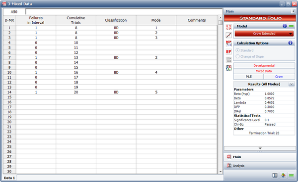
Discrete Mixed Data Example
A one-shot system underwent reliability growth testing for a total of 20 trials. The test was performed as a combination of groups of units with the same configuration and individual trials. The following table shows the data set. The Failures in Interval column specifies the number of failures that occurred in each interval and the Cumulative Trials column specifies the cumulative number of trials at the end of that interval. In other words, the first three rows contain the data from the first trial, in which 8 units with the same configuration were tested and 3 failures (with different failure modes) were observed. The next row contains data from the second trial, in which 2 units with the same configuration were tested and no failures occurred. And so on.
| Mixed Data | |||
| Failures in Interval | Cumulative Trials | Classification | Mode |
|---|---|---|---|
| 1 | 8 | BD | 1 |
| 1 | 8 | BD | 2 |
| 1 | 8 | BD | 3 |
| 0 | 10 | ||
| 0 | 11 | ||
| 0 | 12 | ||
| 1 | 13 | BD | 2 |
| 0 | 14 | ||
| 0 | 15 | ||
| 1 | 16 | BD | 4 |
| 0 | 17 | ||
| 0 | 18 | ||
| 0 | 19 | ||
| 1 | 20 | BD | 5 |
The table also gives the classifications of the failure modes. There are 5 BD modes. The average effectiveness factor for the BD modes is 0.7. Do the following:
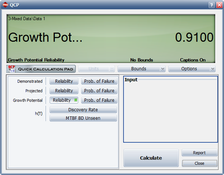
- Calculate the demonstrated reliability at the end of the test.
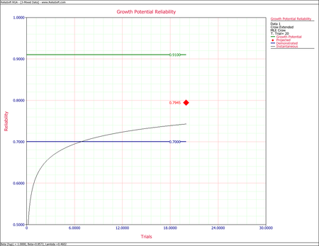
- Calculate the growth potential reliability.
Solution
-
Based on the equations presented in Crow-AMSAA (NHPP), the parameters of the Crow-AMSAA (NHPP) model are estimated as follows:
- [math]\displaystyle{ \widehat{\beta }=0.8572\,\! }[/math]
- [math]\displaystyle{ \widehat{\lambda }=0.4602\,\! }[/math]
- [math]\displaystyle{ \hat{\lambda }=\frac{n}{T_{n}^{\hat{\beta }}}\,\! }[/math]
- [math]\displaystyle{ \begin{align} \hat{\lambda }= & \frac{n}{{{T}_{n}}} \\ = & \frac{6}{20} \\ = & 0.3 \end{align}\,\! }[/math]
- [math]\displaystyle{ \begin{align} {{\lambda }_{i}}(T)=\lambda \beta {{T}^{\beta -1}},\text{with }T\gt 0,\text{ }\lambda \gt 0\text{ and }\beta \gt 0 \end{align}\,\! }[/math]
- [math]\displaystyle{ {{Q}_{i}}(20)=\widehat{\lambda }=0.3\,\! }[/math]
- [math]\displaystyle{ \begin{align} {{R}_{i}}(20)= & 1-{{Q}_{i}}(20) \\ = & 1-0.3 \\ = & 0.7 \end{align}\,\! }[/math]
- The growth potential unreliability is:
- [math]\displaystyle{ \begin{align} {{\widehat{Q}}_{GP}}(T)= & \left( \frac{{{N}_{A}}}{T}+\underset{i=1}{\overset{M}{\mathop \sum }}\,(1-{{d}_{i}})\frac{{{N}_{i}}}{T} \right) \\ = & \underset{i=1}{\overset{M}{\mathop \sum }}\,(1-0.7)\frac{{{N}_{i}}}{T} \\ = & 0.3*(\frac{1+1+1+1+1+1)}{20} \\ = & 0.09 \end{align}\,\! }[/math]
- [math]\displaystyle{ \begin{align} {{\widehat{R}}_{GP}}(T) = & 1-{{\widehat{Q}}_{GP}}(T) \\ = & 1-0.09 \\ = & 0.91 \end{align}\,\! }[/math]


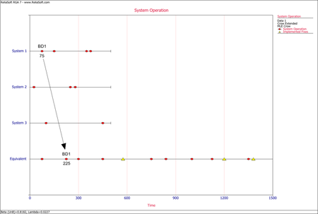
Multiple Systems with Event Codes
Consider the data set shown in the following figure.

Solution
The first step to creating the equivalent system is to isolate each failure mode and its implemented fixes independently from each other. The numbered steps follow the five rules and are presented in the same numbering sequence.
- The next figure illustrates the application of rule #1 for mode BD1. The mode in the equivalent single system is calculated as [math]\displaystyle{ (75+75+75)=225\,\! }[/math] or [math]\displaystyle{ 75*3=225.\,\! }[/math]
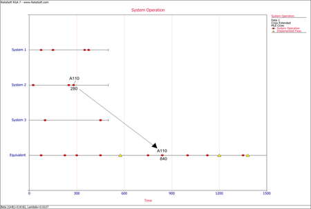
The next figure illustrates the application of rule #1 for mode A110. The mode in the equivalent single system is calculated as [math]\displaystyle{ (280+280+280)=840\,\! }[/math] or [math]\displaystyle{ 280*3=840.\,\! }[/math]
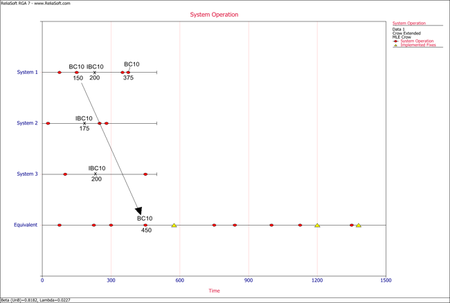
- The next figure illustrates the application of rule #2 for the first occurrence of the mode BC10 in system 1. The mode in the equivalent single system is calculated as [math]\displaystyle{ (150+150+150)=450\,\! }[/math] or [math]\displaystyle{ 150*3=450.\,\! }[/math]
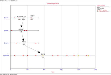
- The next figure illustrates the application of rule #3 for implemented fixes (I events) of the mode BC10. In the graph, the I events are symbolized by having the letter "I" before the naming of the mode. In this case, IBC10 is for the implemented fix of mode BC10. The IBC10 in the equivalent single system is calculated as [math]\displaystyle{ (200+175+200)=575\,\! }[/math].
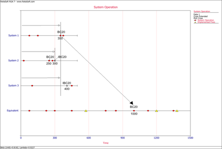
- The next figure illustrates the application of rule #4 for the mode BC20 in system 1, which occurs after a fix for the same mode was implemented in system 2. The mode in the equivalent single system is calculated as [math]\displaystyle{ (350+300+350)=1000.\,\! }[/math]
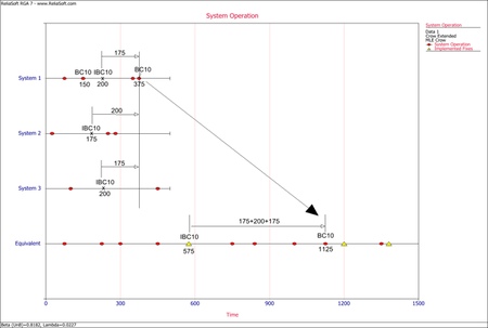
- The next figure illustrates the application of rule #5 for the second occurrence of the mode BC10 in system 1, which occurs after an implemented fix (I event) has occurred for that mode in the same system. The mode in the equivalent single system is calculated as [math]\displaystyle{ 575+(175+200+175)=1125.\,\! }[/math]
After having transferred the data set to the Crow Extended equivalent system, the data set is analyzed using the Crow Extended model. The last figure shows the growth potential MTBF plot.


Multiple Systems - Concurrent Operating Times
Three systems were subjected to a reliability growth test to evaluate the prototype of a new product. Based on a failure analysis on the results of the test, the proposed management strategy is to delay corrective actions until after the test. The tables shown next display the data set and the associated effectiveness factors for the unique BD modes.
| Multiple Systems (Concurrent Operating Times) Data | |||
| System 1 | System 2 | System 3 | |
|---|---|---|---|
| Start Time | 0 | 0 | 0 |
| End Time | 541 | 454 | 436 |
| Times-to-Failure | 83 BD37 | 26 BD25 | 23 BD30 |
| 83 BD43 | 26 BD43 | 46 BD49 | |
| 83 BD46 | 57 BD37 | 127 BD47 | |
| 169 A45 | 64 BD19 | 166 A2 | |
| 213 A18 | 169 A45 | 169 BD23 | |
| 299 A42 | 213 A32 | 213 BD7 | |
| 375 A1 | 231 BD8 | 213 BD29 | |
| 431 BD16 | 231 BD25 | 255 BD26 | |
| 231 BD27 | 369 A33 | ||
| 231 A28 | 374 BD29 | ||
| 304 BD24 | 380 BD22 | ||
| 383 BD40 | 415 BD7 | ||
| Effectiveness factors | |
| BD Mode | Effectiveness Factor |
|---|---|
| 30 | 0.75 |
| 43 | 0.5 |
| 25 | 0.5 |
| 49 | 0.75 |
| 37 | 0.9 |
| 19 | 0.75 |
| 46 | 0.75 |
| 47 | 0.25 |
| 23 | 0.5 |
| 7 | 0.25 |
| 29 | 0.25 |
| 8 | 0.5 |
| 27 | 0.5 |
| 26 | 0.75 |
| 24 | 0.5 |
| 22 | 0.5 |
| 40 | 0.75 |
| 16 | 0.75 |
The prototype is required to meet a projected MTBF goal of 55 hours. Do the following:
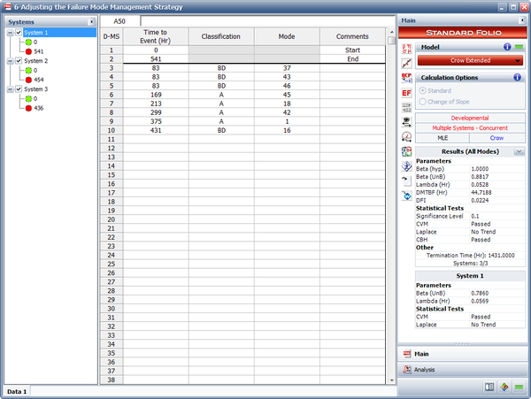
- Estimate the parameters of the Crow Extended model.
- Based on the current management strategy what is the projected MTBF?
- If the projected MTBF goal is not met, alter the current management strategy to meet this requirement with as little adjustment as possible and without changing the EFs of the existing BD modes. Assume an EF = 0.7 for any newly assigned BD modes.
Solution
- The next figure shows the estimated Crow Extended parameters.
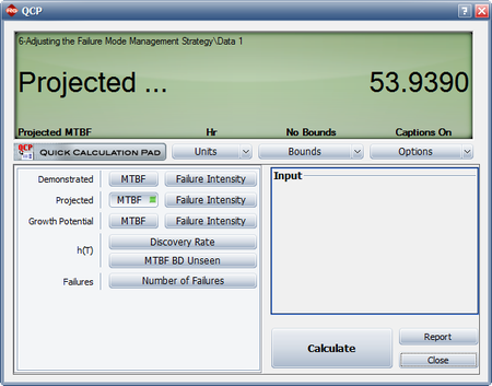
- There are a couple of ways to calculate the projected MTBF, but the easiest is via the Quick Calculation Pad (QCP). The following result shows that the projected MTBF is estimated to be 53.9390 hours, which is below the goal of 55 hours.
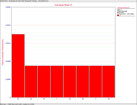
- To reach our goal, or to see if we can even get there, the management strategy must be changed. The effectiveness factors for the existing BD modes cannot be changed; however, it is possible to change an A mode to a BD mode, but which A mode(s) should be changed? To answer this question, create an Individual Mode Failure Intensity plot with just the A modes displayed, as shown next. As you can see from the plot, failure mode A45 has the highest failure intensity. Therefore, among the A modes, this particular failure mode has the greatest negative effect on the system MTBF.
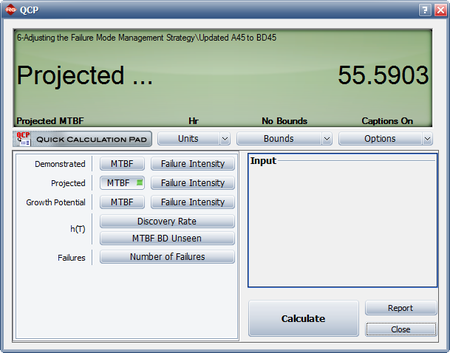
Change A45 to BD45. Be sure to change all instances of A45 to a BD mode. Enter an effectiveness factor of 0.7 for BD45, and then recalculate the parameters of the Crow Extended model. Now go back to the QCP to calculate the projected MTBF, as shown below. The projected MTBF is now estimated to be 55.5903 hours. Based on the change in the management strategy, the projected MTBF goal is now expected to be met.


Multiple Systems - Known Operating Times
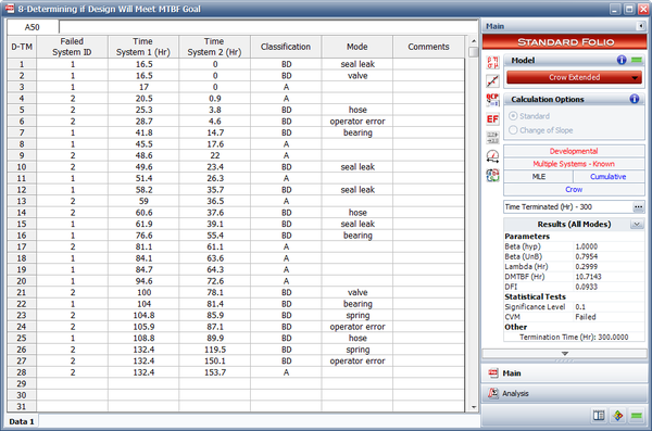
Two prototypes of a new design are tested simultaneously. Whenever a failure is observed for one unit, the current operating time of the other unit is also recorded. The test is terminated after 300 hours. All of the design changes for the prototypes were delayed until after completing the test. The data set is given in the table below. Assume a fixed effectiveness factor equal to 0.7. The MTBF goal for the new design is 30 hours. Do the following:
- Estimate the parameters of the Crow Extended model.
- What is the projected MTBF and growth potential?
- Under the current management strategy, is it even possible to reach the MTBF goal of 30 hours?
| Multiple Systems (Known Operating Times) Data | ||||
| Failed Unit ID | Time Unit 1 | Time Unit 2 | Classification | Mode |
|---|---|---|---|---|
| 1 | 16.5 | 0 | BD | seal leak |
| 1 | 16.5 | 0 | BD | valve |
| 1 | 17 | 0 | A | |
| 2 | 20.5 | 0.9 | A | |
| 2 | 25.3 | 3.8 | BD | hose |
| 2 | 28.7 | 4.6 | BD | operator error |
| 1 | 41.8 | 14.7 | BD | bearing |
| 1 | 45.5 | 17.6 | A | |
| 2 | 48.6 | 22 | A | |
| 2 | 49.6 | 23.4 | BD | seal leak |
| 1 | 51.4 | 26.3 | A | |
| 1 | 58.2 | 35.7 | BD | seal leak |
| 2 | 59 | 36.5 | A | |
| 2 | 60.6 | 37.6 | BD | hose |
| 1 | 61.9 | 39.1 | BD | seal leak |
| 1 | 76.6 | 55.4 | BD | bearing |
| 2 | 81.1 | 61.1 | A | |
| 1 | 84.1 | 63.6 | A | |
| 1 | 84.7 | 64.3 | A | |
| 1 | 94.6 | 72.6 | A | |
| 2 | 100 | 78.1 | BD | valve |
| 1 | 104 | 81.4 | BD | bearing |
| 2 | 104.8 | 85.9 | BD | spring |
| 2 | 105.9 | 87.1 | BD | operator error |
| 1 | 108.8 | 89.9 | BD | hose |
| 2 | 132.4 | 119.5 | BD | spring |
| 2 | 132.4 | 150.1 | BD | operator error |
| 2 | 132.4 | 153.7 | A | |
Solution
- The next figure shows the estimated Crow Extended parameters.
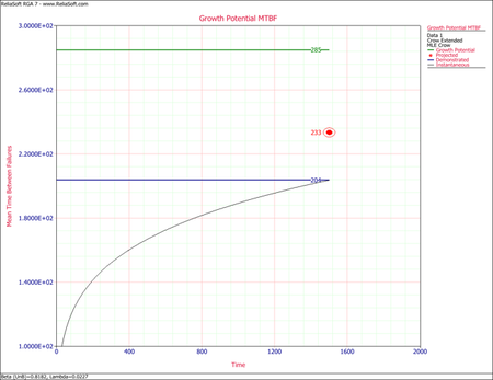
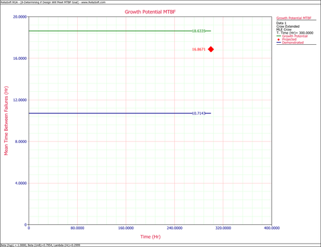
- One possible method for calculating the projected MTBF and growth potential is to use the Quick Calculation Pad, but you can also view these two values at the same time by viewing the Growth Potential MTBF plot, as shown next. From the plot, the projected MTBF is equal to 16.87 hours and the growth potential is equal to 18.63 hours.
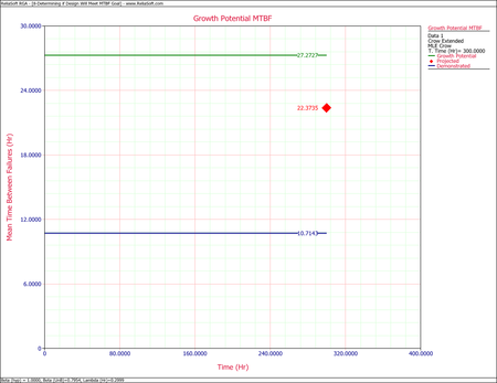
- The current projected MTBF and growth potential MTBF are both well below the required goal of 30 hours. To check if this goal can even be reached, you can set the effectiveness factor equal to 1. In other words, if all of the corrective actions were to remove the failure modes completely, what would be the projected and growth potential MTBF?
Change the fixed effectiveness factor to 1, then recalculate the parameters and refresh the Growth Potential plot, as shown next. Even if you assume an effectiveness factor equal to 1, the growth potential is still only 27.27 hours. Based on the current design process, it will not be possible to reach the MTBF goal of 30 hours. Therefore, you have two options: start a new design stage or reduce the required MTBF goal.


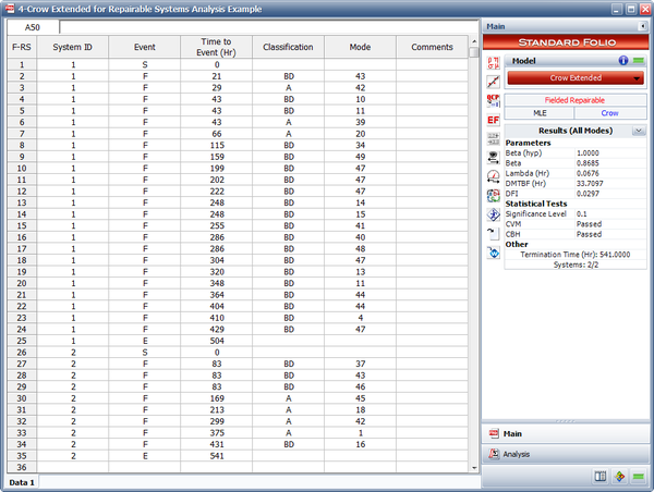
Repairable System Example
The failures and fixes of two repairable systems in the field are recorded. Both systems started operating from time 0. System 1 ends at time = 504 and system 2 ends at time = 541. All the BD modes are fixed at the end of the test. A fixed effectiveness factor equal to 0.6 is used. Answer the following questions:
- Estimate the parameters of the Crow Extended model.
- Calculate the projected MTBF after the delayed fixes.
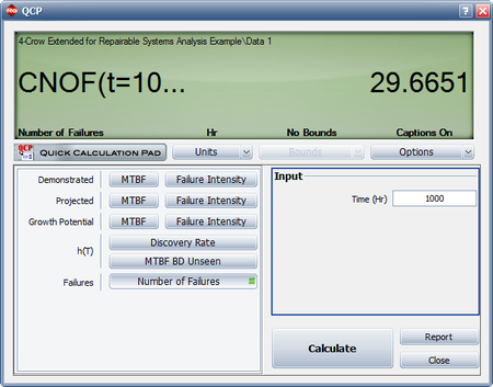
- If no fixes were performed for the future failures, what would be the expected number of failures at time 1,000?
Solution
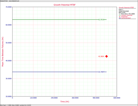
- The next figure shows the estimated Crow Extended parameters.
- The next figure shows the projected MTBF at time = 541 (i.e., the age of the oldest system).
- The next figure shows the expected number of failures at time = 1,000.


Fleet Analysis Examples
Example 1
The following table presents data for a fleet of 27 systems. A cycle is a complete history from overhaul to overhaul. The failure history for the last completed cycle for each system is recorded. This is a random sample of data from the fleet. These systems are in the order in which they were selected. Suppose the intervals to group the current data are 10,000; 20,000; 30,000; 40,000 and the final interval is defined by the termination time. Conduct the fleet analysis.
| Sample Fleet Data | |||
| System | Cycle Time [math]\displaystyle{ {{T}_{j}}\,\! }[/math] | Number of failures [math]\displaystyle{ {{N}_{j}}\,\! }[/math] | Failure Time [math]\displaystyle{ {{X}_{ij}}\,\! }[/math] |
|---|---|---|---|
| 1 | 1396 | 1 | 1396 |
| 2 | 4497 | 1 | 4497 |
| 3 | 525 | 1 | 525 |
| 4 | 1232 | 1 | 1232 |
| 5 | 227 | 1 | 227 |
| 6 | 135 | 1 | 135 |
| 7 | 19 | 1 | 19 |
| 8 | 812 | 1 | 812 |
| 9 | 2024 | 1 | 2024 |
| 10 | 943 | 2 | 316, 943 |
| 11 | 60 | 1 | 60 |
| 12 | 4234 | 2 | 4233, 4234 |
| 13 | 2527 | 2 | 1877, 2527 |
| 14 | 2105 | 2 | 2074, 2105 |
| 15 | 5079 | 1 | 5079 |
| 16 | 577 | 2 | 546, 577 |
| 17 | 4085 | 2 | 453, 4085 |
| 18 | 1023 | 1 | 1023 |
| 19 | 161 | 1 | 161 |
| 20 | 4767 | 2 | 36, 4767 |
| 21 | 6228 | 3 | 3795, 4375, 6228 |
| 22 | 68 | 1 | 68 |
| 23 | 1830 | 1 | 1830 |
| 24 | 1241 | 1 | 1241 |
| 25 | 2573 | 2 | 871, 2573 |
| 26 | 3556 | 1 | 3556 |
| 27 | 186 | 1 | 186 |
| Total | 52110 | 37 | |
Solution
The sample fleet data set can be grouped into 10,000; 20,000; 30,000; 40,000 and 52,110 time intervals. The following table gives the grouped data.
| Grouped Data | |
| Time | Observed Failures |
|---|---|
| 10,000 | 8 |
| 20,000 | 16 |
| 30,000 | 22 |
| 40,000 | 27 |
| 52,110 | 37 |
Based on the above time intervals, the maximum likelihood estimates of [math]\displaystyle{ \widehat{\lambda }\,\! }[/math] and [math]\displaystyle{ \widehat{\beta }\,\! }[/math] for this data set are then given by:
- [math]\displaystyle{ \begin{matrix} \widehat{\lambda }=0.00147 \\ \widehat{\beta }=0.93328 \\ \end{matrix}\,\! }[/math]
The next figure shows the System Operation plot.

Example 2
11 systems from the field were chosen for fleet analysis. Each system had at least one failure. All of the systems had a start time equal to zero and the last failure for each system corresponds to the end time. Group the data based on a fixed interval of 3,000 hours, and assume a fixed effectiveness factor equal to 0.4. Do the following:
- Estimate the parameters of the Crow Extended model.
- Based on the analysis, does it appear that the systems were randomly ordered?
- After the implementation of the delayed fixes, how many failures would you expect within the next 4,000 hours of fleet operation.
| Fleet Data | |
| System | Times-to-Failure |
|---|---|
| 1 | 1137 BD1, 1268 BD2 |
| 2 | 682 BD3, 744 A, 1336 BD1 |
| 3 | 95 BD1, 1593 BD3 |
| 4 | 1421 A |
| 5 | 1091 A, 1574 BD2 |
| 6 | 1415 BD4 |
| 7 | 598 BD4, 1290 BD1 |
| 8 | 1556 BD5 |
| 9 | 55 BD4 |
| 10 | 730 BD1, 1124 BD3 |
| 11 | 1400 BD4, 1568 A |
Solution
- The next figure shows the estimated Crow Extended parameters.
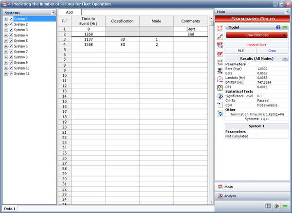
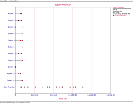
- Upon observing the estimated parameter [math]\displaystyle{ \beta \,\! }[/math], it does appear that the systems were randomly ordered since [math]\displaystyle{ \beta =0.8569\,\! }[/math]. This value is close to 1. You can also verify that the confidence bounds on [math]\displaystyle{ \beta \,\! }[/math] include 1 by going to the QCP and calculating the parameter bounds or by viewing the Beta Bounds plot. However, you can also determine graphically if the systems were randomly ordered by using the System Operation plot as shown below. Looking at the Cum. Time Line, it does not appear that the failures have a trend associated with them. Therefore, the systems can be assumed to be randomly ordered.
- After implementing the delayed fixes, the system's projected MTBF is equal to [math]\displaystyle{ 1035.6802\,\! }[/math] as shown in the plot below.
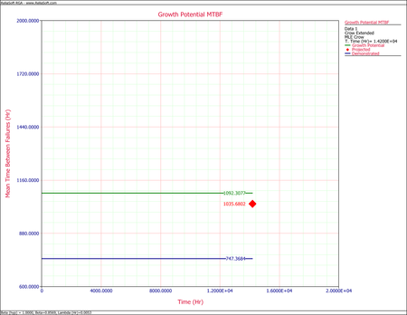
To estimate the number of failures during the next 4,000 hours, calculate the following:
[math]\displaystyle{ \begin{align} N=& \frac{4000}{1035.6802}\\ = & 3.8622\end{align}\,\! }[/math]
Therefore, it is estimated that [math]\displaystyle{ \approx\,\! }[/math] 4 failures will be observed during the next 4,000 hours of fleet operation.


