Template:Weibull parameters probability plotting
Probability Plotting
One method of calculating the parameters of the Weibull distribution is by using probability plotting. To better illustrate this procedure, consider the following example from Kececioglu [20].
Probability Plotting Example
Assume that six identical units are being reliability tested at the same application and operation stress levels. All of these units fail during the test after operating the following number of hours, Ti: 93, 34, 16, 120, 53 and 75. Estimate the values of the parameters for a two-parameter Weibull distribution and determine the reliability of the units at a time of 15 hours.
Probability Plotting Example Solution
The steps for determining the parameters of the Weibull representing the data, using probability plotting, are outlined in the following instructions. First, rank the times-to-failure in ascending order as shown next.
| Time-to-failure, hrs |
Failure Order Number out of Sample Size of 6 |
|---|---|
| 16 | 1 |
| 34 | 2 |
| 53 | 3 |
| 75 | 4 |
| 93 | 5 |
| 120 | 6 |
Obtain their median rank plotting positions. Median rank positions are used instead of other ranking methods because median ranks are at a specific confidence level (50%). Median ranks can be found tabulated in many reliability books. They can also be estimated using the following equation,
- [math]\displaystyle{ MR \sim { \frac{i-0.3}{N+0.4}}\cdot 100, }[/math]
where [math]\displaystyle{ i }[/math] is the failure order number and [math]\displaystyle{ N }[/math] is the total sample size. The exact median ranks are found in Weibull++ by solving,
- [math]\displaystyle{ \sum_{k=i}^N{\binom{N}{k}}{MR^k}{(1-MR)^{N-k}}=0.5=50% }[/math]
for [math]\displaystyle{ MR }[/math], where [math]\displaystyle{ N }[/math] is the sample size and [math]\displaystyle{ i }[/math] the order number. The times-to-failure, with their corresponding median ranks, are shown next.
| Time-to-failure, hrs | Median Rank,% |
|---|---|
| 16 | 10.91 |
| 34 | 26.44 |
| 53 | 42.14 |
| 75 | 57.86 |
| 93 | 73.56 |
| 120 | 89.1 |
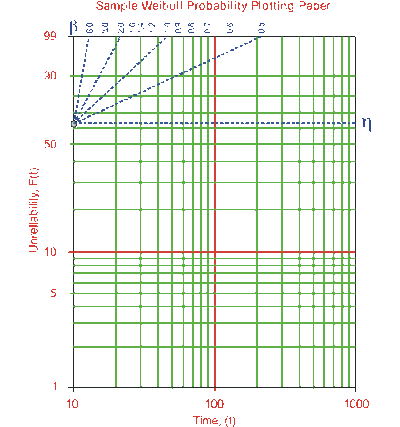
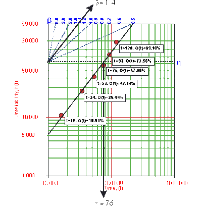
On a Weibull probability paper, plot the times and their corresponding ranks. A sample of a Weibull probability paper is given in Figure 6-7 and the plot of the data in the example in Figure 6-8.
Draw the best possible straight line through these points, as shown below, then obtain the slope of this line by drawing a line, parallel to the one just obtained, through the slope indicator. This value is the estimate of the shape parameter [math]\displaystyle{ \hat{\beta } }[/math], in this case [math]\displaystyle{ \hat{\beta }=1.4 }[/math].
At the [math]\displaystyle{ Q(t)=63.2% }[/math] ordinate point, draw a straight horizontal line until this line intersects the fitted straight line. Draw a vertical line through this intersection until it crosses the abscissa. The value at the intersection of the abscissa is the estimate of [math]\displaystyle{ \hat{\eta } }[/math]. For this case, [math]\displaystyle{ \hat{\eta }=76 }[/math] hours. (This is always at 63.2% since: [math]\displaystyle{ Q(T)=1-e^{-(\frac{\eta }{\eta })^{\beta }}=1-e^{-1}=0.632=63.2% }[/math].
Now any reliability value for any mission time [math]\displaystyle{ t }[/math] can be obtained. For example, the reliability for a mission of 15 hours, or any other time, can now be obtained either from the plot or analytically. To obtain the value from the plot, draw a vertical line from the abscissa, at hours, to the fitted line. Draw a horizontal line from this intersection to the ordinate and read Q(t), in this case [math]\displaystyle{ Q(t)=9.8% }[/math]. Thus, [math]\displaystyle{ R(t)=1-Q(t)=90.2% }[/math]. This can also be obtained analytically from the Weibull reliability function since the estimates of both of the parameters are known or:
[math]\displaystyle{ R(t=15)=e^{-\left( \frac{15}{\eta }\right) ^{\beta }}=e^{-\left( \frac{15}{76 }\right) ^{1.4}}=90.2% }[/math]
Probability Plotting for the Location Parameter, γ
The third parameter of the Weibull distribution is utilized when the data do not fall on a straight line, but fall on either a concave up or down curve. The following statements can be made regarding the value of γ:
- Case 1: If the curve for MR versus Tj is concave down and the curve for MR versus (Tj − T1) is concave up, then there exists a γ such that 0 < γ < T1, or γ has a positive value.
- Case 2: If the curves for MR versus Tj and MR versus (Tj − T1) are both concave up, then there exists a negative γ which will straighten out the curve of MR versus Tj.
- Case 3: If neither one of the previous two cases prevails, then either reject the Weibull as one capable of representing the data, or proceed with the multiple population (mixed Weibull) analysis. To obtain the location parameter, γ:
- Subtract the same arbitrary value, γ, from all the times to failure and replot the data.
- If the initial curve is concave up, subtract a negative γ from each failure time.
- If the initial curve is concave down, subtract a positive γ from each failure time.
- Repeat until the data plots on an acceptable straight line.
- The value of γ is the subtracted (positive or negative) value that places the points in an acceptable straight line.
The other two parameters are then obtained using the techniques previously described. Also, it is important to note that we used the term subtract a positive or negative gamma, where subtracting a negative gamma is equivalent to adding it. Note that when adjusting for gamma, the x-axis scale for the straight line becomes (T − γ).
Three-parameter Weibull distribution example
Six identical units are reliability tested under the same stresses and conditions. All units are tested to failure and the following times-to-failure are recorded: 48, 66, 85, 107, 125 and 152 hours. Find the parameters of the three-parameter Weibull distribution using probability plotting.
Solution
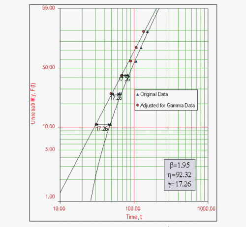
The following figure shows the results. Note that since the original data set was concave down, 17.26 was subtracted from all the times-to-failure and replotted, resulting in a straight line, thus γ = 17.26. (We used Weibull++ to get the results. To perform this by hand, one would attempt different values of γ, using a trial and error methodology, until an acceptable straight line is found. When performed manually, you do not expect decimal accuracy.)


