Template:Weibull++ Equation Fit Solver Example: Difference between revisions
No edit summary |
No edit summary |
||
| Line 32: | Line 32: | ||
|} | |} | ||
From the physical mechanism, the engineer knows the degradation path follows the following equation: | |||
::<math>y=a+bx+c\ln (x)</math> | |||
where: | |||
• x is the time | |||
• y is the degradation reading. | |||
This above model is not a standard degradation model in Webul++. It can be solved using the equation fit solver. | |||
'''Solution:''' | |||
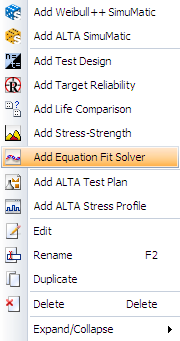
'''Step 1:''' Create an Equation Fit Solver Folio | |||
[[Image: Select Equation Fit Solver.png|thumb|center|400px]] | |||
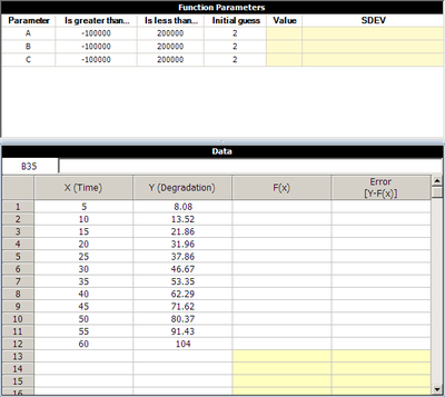
'''Step 2:''' Enter the above data into the folio | |||
[[Image: Equation Fit Solver Data.png|thumb|center|400px]] | |||
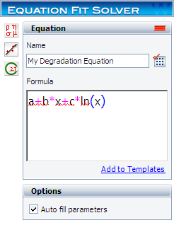
'''Step 3:''' Enter the user defined degradation function at the control panel and name it “My Degradation Equation”. | |||
[[Image: Equation Fit Solver Function.png|thumb|center|400px]] | |||
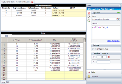
'''Step 4:''' Calculate it and the results are: | |||
[[Image: Equation Fit Solver Result.png|thumb|center|400px]] | |||
'''Step 5:''' You can use the “Calculate Y given X” to make prediction. For example, the predicted Y value at X=100 is 176.2424. | |||
[[Image: Equation Fit Solver Prediction.png|thumb|center|400px]] | |||
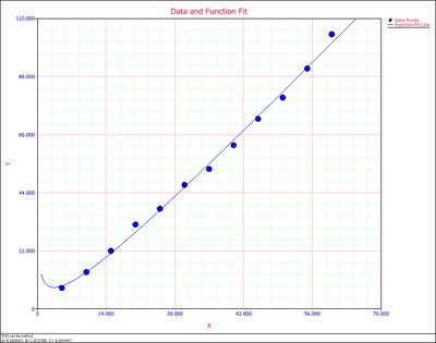
'''Step 6:'' The plot of the fitted model and the observed values are given as: | |||
[[Image: Equation Fit Solver Plot.png|thumb|center|400px]] | |||
Revision as of 17:24, 7 March 2012
Weibull++ Equation Fit Solver Example
Equation Fit Solver can be used to do linear and nonlinear regression. Assume an engineer collected the following degradation data.
| Time | Reading |
| 5 | 8.08 |
| 10 | 13.52 |
| 15 | 21.86 |
| 20 | 31.96 |
| 25 | 37.86 |
| 30 | 46.67 |
| 35 | 53.35 |
| 40 | 62.29 |
| 45 | 71.62 |
| 50 | 80.37 |
| 55 | 91.43 |
| 60 | 104.00 |
From the physical mechanism, the engineer knows the degradation path follows the following equation:
- [math]\displaystyle{ y=a+bx+c\ln (x) }[/math]
where: • x is the time • y is the degradation reading. This above model is not a standard degradation model in Webul++. It can be solved using the equation fit solver.
Solution:
Step 1: Create an Equation Fit Solver Folio
Step 2: Enter the above data into the folio
Step 3: Enter the user defined degradation function at the control panel and name it “My Degradation Equation”.
Step 4: Calculate it and the results are:
Step 5: You can use the “Calculate Y given X” to make prediction. For example, the predicted Y value at X=100 is 176.2424.
'Step 6: The plot of the fitted model and the observed values are given as:
