Template:Example: 2P Weibull Distribution RRX: Difference between revisions
Jump to navigation
Jump to search
No edit summary |
No edit summary |
||
| Line 40: | Line 40: | ||
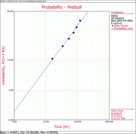
The results and the associated graph using Weibull++ are given next. Note that the slight variation in the results is due to the number of significant figures used in the estimation of the median ranks. Weibull++ by default uses double precision accuracy when computing the median ranks. | The results and the associated graph using Weibull++ are given next. Note that the slight variation in the results is due to the number of significant figures used in the estimation of the median ranks. Weibull++ by default uses double precision accuracy when computing the median ranks. | ||
[[Image:Weibull Distribution Example 4 RRX Plot.png | [[Image:Weibull Distribution Example 4 RRX Plot.png|center|450px| ]] | ||
<br> | <br> | ||
Revision as of 05:38, 6 August 2012
2P Weibull Distribution RRX Example
Repeat Example 1 using rank regression on X.
Solution
The Table constructed in Example 3, can also be applied to this example.
Using the values from this table we get:
- [math]\displaystyle{ \hat{b} ={\frac{\sum\limits_{i=1}^{6}(\ln T_{i})y_{i}-\frac{ \sum\limits_{i=1}^{6}\ln T_{i}\sum\limits_{i=1}^{6}y_{i}}{6}}{ \sum\limits_{i=1}^{6}y_{i}^{2}-\frac{\left( \sum\limits_{i=1}^{6}y_{i}\right) ^{2}}{6}}} }[/math]
- [math]\displaystyle{ \hat{b} =\frac{-8.0699-(23.9068)(-3.0070)/6}{7.1502-(-3.0070)^{2}/6} }[/math]
or:
- [math]\displaystyle{ \hat{b}=0.6931 }[/math]
and:
- [math]\displaystyle{ \hat{a}=\overline{x}-\hat{b}\overline{y}=\frac{\sum\limits_{i=1}^{6}\ln T_{i} }{6}-\hat{b}\frac{\sum\limits_{i=1}^{6}y_{i}}{6} }[/math]
or:
- [math]\displaystyle{ \hat{a}=\frac{23.9068}{6}-(0.6931)\frac{(-3.0070)}{6}=4.3318 }[/math]
Therefore:
- [math]\displaystyle{ \hat{\beta }=\frac{1}{\hat{b}}=\frac{1}{0.6931}=1.4428 }[/math]
and:
- [math]\displaystyle{ \hat{\eta }=e^{\frac{\hat{a}}{\hat{b}}\cdot \frac{1}{\hat{ \beta }}}=e^{\frac{4.3318}{0.6931}\cdot \frac{1}{1.4428}}=76.0811\text{ hr} }[/math]
The correlation coefficient is:
- [math]\displaystyle{ \hat{\rho }=0.9956 }[/math]
The results and the associated graph using Weibull++ are given next. Note that the slight variation in the results is due to the number of significant figures used in the estimation of the median ranks. Weibull++ by default uses double precision accuracy when computing the median ranks.
