Template:Difference detection matrix
Test Design Using a Life Difference Detection Matrix
Engineers often need to design tests for detecting life differences between two or more product designs. The questions are how many samples and how long should the test be conducted in order to detect a certain amount of difference. There are no simple answers. Usually, advanced design of experiments (DOE) techniques should be utilized. For a simple case, such as comparing two designs, the Difference Detection Matrix in Weibull++ can be used. The difference detection matrix graphically indicates the amount of test time required to detect a statistical difference in the lives of two populations.
As discussed in the test design using expected failure times plot, if the sample size is known, the expected failure time of each test unit can be obtained based on the assumed failure distribution. Now let's go one step further. With these failure times, we can then estimate the failure distribution and calculate any reliability metrics. This process is similar to the simulation used in Simumatic where random failure times are generated from simulation and then used to estimate the failure distribution. This approach is also used by the difference detection matrix.
Assume we want to compare the B10 lifes (or mean lifes) of two designs. The test is time-terminated and the termination time is set to T. Using the method given in Test Design Using Expected Failure Time Plots, we can generate the failure times. For any failure time greater than T, it is a suspension and the suspension time is T. For each design, its B10 life and confidence bounds can be estimated from the generated failure/suspension times. If the two estimated confidence intervals overlap with each other, it means the difference of the two B10 lifes cannot be detected from this test. We have to either increase the sample size or the test duration.
Example 7:
In this example, you will use the Difference Detection Matrix to choose the suitable sample size and duration for a reliability test. Assume that there are two design options for a new product. The engineers need to design a test that compares the reliability performance of these two options. The reliability for both designs is assumed to follow a Weibull distribution. For Design 1, its shape parameter [math]\displaystyle{ \beta = 3\,\! }[/math]; for Design 2, its [math]\displaystyle{ \beta= 2\,\! }[/math]. Their B10 lives may range from 500 to 3,000 hours.
Solution
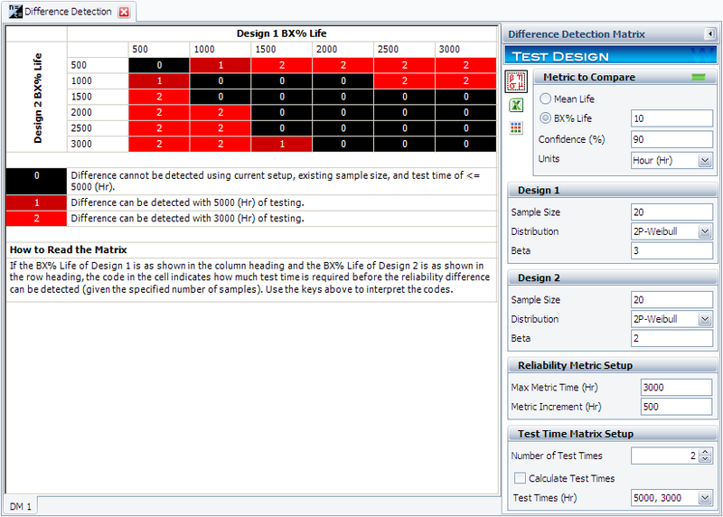
For the initial setup, set the sample size for each design to 20, and use two test durations of 3,000 and 5,000 hours. The following picture shows the complete control panel setup and the results of the analysis.
The columns in the matrix show the range of the assumed B10 life for design 1, while the rows show the range for design 2. A value of 0 means the difference cannot be detected through the test, 1 means the difference can be detected if the test duration is 5,000 hours, and 2 means the difference can be detected if the test duration is 3,000 hours. For example, the number is 2 for cell (1000, 2000). This means that if the B10 life for Design 1 is 1,000 hours and the B10 life for Design 2 is 2,000 hours, the difference can be detected if the test duration is at least 5,000 hours.
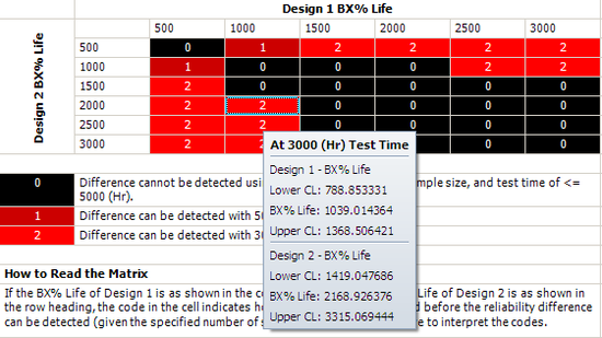
Click inside the cell to show the estimated confidence intervals, as shown next. By testing 20 samples each for 3,000 hours, the difference of their B10 lives probably can be detected. This is because, at a confidence level of 90%, the estimated confidence intervals on the B10 life do not overlap.
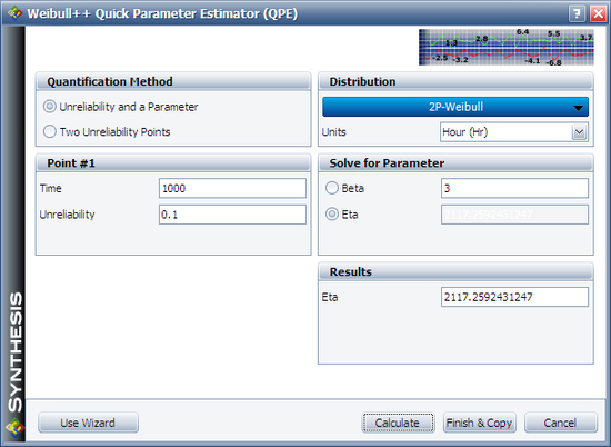
We will use Design 1 to illustrate how the interval is calculated. For cell (1000, 2000), Design 1's B10 life is 1,000 and the assumed [math]\displaystyle{ \beta\,\! }[/math] is 3. We can calculate the [math]\displaystyle{ \eta\,\! }[/math] for the Weibull distribution using the Quick Parameter Estimator tool, as shown next.
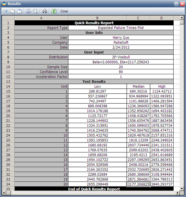
The estimated [math]\displaystyle{ \eta\,\! }[/math] is 2117.2592 hours. We can then use these distribution parameters and the sample size of 20 to get the expected failure times by using Weibull's Expected Failure Times Plot. The following report shows the result from that utility.
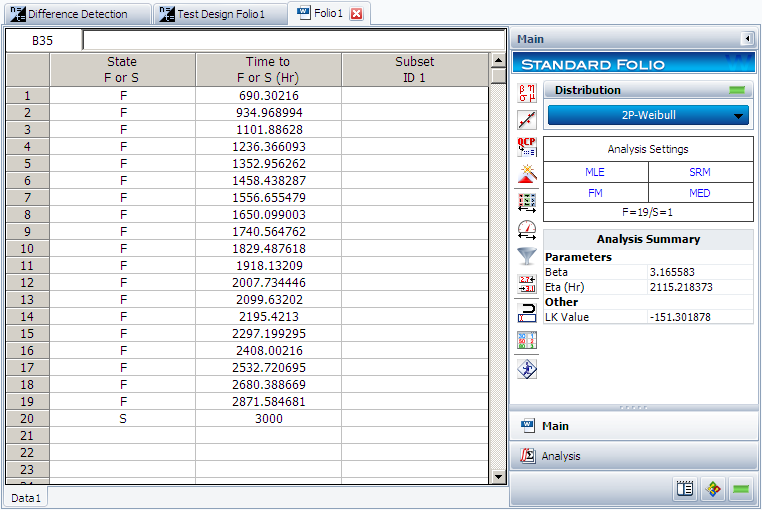
The median failure times are used to estimate the failure distribution. Note that since the test duration is set to 3,000 hours, any failures that occur after 3,000 are treated as suspensions. In this case, the last failure is a suspension with a suspension time of 3,000 hours. We can enter the median failure times data set into a standard Weibull++ folio as given in the next figure.
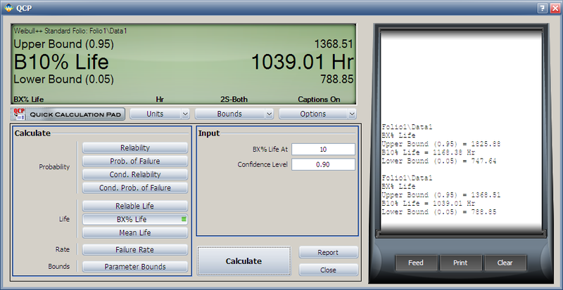
After analyzing the data set with the MLE and FM analysis options, we can now calculate the B10 life and its interval in the QCP, as shown next.
From this result, we can see that the estimated B10 life and its confidence intervals are the same as the results displayed in the Difference Detection Matrix.
The above procedure can be repeated to get the results for the other cells and for Design 2. Therefore, by adjusting the sample size and test duration, a suitable test time can be identified for detecting a certain amount of difference between two designs/populations.
