Reliability Test Design
Quite often, there is a desire to design reliability demonstration tests that have few or no failures. These tests are often required to demonstrate customer reliability and confidence requirements. While it is desirable to be able to test a large population of units to failure in order to obtain information on a design's reliability, time and resource constraints sometimes make this impossible. In these cases, a test can be run on a specified number of units for a specified amount of time that will demonstrate that the product has met or exceeded a given reliability at a given confidence level. In order to do so without a large amount of cumulative test time or failure data, it is necessary to make assumptions about the failure distribution of the product. In the final analysis, the actual reliability of the units will, of course, remain unknown, but the reliability engineer will be able to state that certain specifications have been met.
Demonstration Test Design
Frequently, a manufacturer will have to demonstrate that a certain product has met a goal of a certain reliability at a given time with a specific confidence. Often, it will be desired to demonstrate that this goal has been met with a zero-failure test. In order to design and conduct such a test, something about the failure behavior of the product will need to be known (i.e., the shape parameter of the product's life distribution). Beyond this, nothing more about the test is known, and usually the engineer designing the test will have to study the financial trade-offs between the number of units and the amount of test time needed to demonstrate the desired goal. In cases like this, it is useful to have a "carpet plot" that shows the possibilities of how a certain specification can be met.
This methodology requires the use of the cumulative binomial distribution in addition to the assumed distribution of the product's lifetimes. Not only does the life distribution of the product need to be assumed beforehand, but a reasonable assumption of the distribution's shape parameter must be provided as well. Additional information that must be supplied includes: a) the reliability to be demonstrated, b) the confidence level at which the demonstration takes place, c) the acceptable number of failures and d) either the number of available units or the amount of available test time. The output of this analysis can be the amount of time required to test the available units or the required number of units that need to be tested during the available test time.
Reliability Demonstration
Frequently, the entire purpose of designing a test with few or no failures is to demonstrate a certain reliability, [math]\displaystyle{ {{R}_{DEMO}} }[/math], at a certain time. With the exception of the exponential distribution (and ignoring the location parameter for the time being), this reliability is going to be a function of time, a shape parameter and a scale parameter.
where:
- [math]\displaystyle{ {{t}_{DEMO}} }[/math] is the time at which the demonstrated reliability is specified.
- [math]\displaystyle{ \theta }[/math] is the shape parameter.
- [math]\displaystyle{ \phi }[/math] is the scale parameter.
Since required inputs to the process include [math]\displaystyle{ {{R}_{DEMO}} }[/math], [math]\displaystyle{ {{t}_{DEMO}} }[/math] and [math]\displaystyle{ \theta }[/math], the value of the scale parameter can be backed out of the reliability equation of the assumed distribution, and will be used in the calculation of another reliability value, [math]\displaystyle{ {{R}_{TEST}} }[/math], which is the reliability that is going to be incorporated into the actual test calculation. How this calculation is performed depends on whether one is attempting to solve for the number of units to be tested in an available amount of time, or attempting to determine how long to test an available number of test units.
Determining Units for Available Test Time
If one knows that the test is to last a certain amount of time, [math]\displaystyle{ {{t}_{TEST}} }[/math], the number of units that must be tested to demonstrate the specification must be determined. The first step in accomplishing this involves calculating the [math]\displaystyle{ {{R}_{TEST}} }[/math] value.
This should be a simple procedure since:
and [math]\displaystyle{ {{t}_{DEMO}} }[/math], [math]\displaystyle{ \theta }[/math] and [math]\displaystyle{ \phi }[/math] are already known, and it is just a matter of plugging these values into the appropriate reliability equation.
We now incorporate a form of the cumulative binomial distribution in order to solve for the required number of units. This form of the cumulative binomial appears as:
where:
- [math]\displaystyle{ \begin{align} & CL= \text{the required confidence level} \\ & f= \text{the allowable number of failures} \\ & n= \text{the total number of units on test} \\ & {{R}_{TEST}}= \text{the reliability on test} \end{align} }[/math]
Since [math]\displaystyle{ CL }[/math] and [math]\displaystyle{ f }[/math] are required inputs to the process and [math]\displaystyle{ {{R}_{TEST}} }[/math] has already been calculated, it merely remains to solve the cumulative binomial equation for [math]\displaystyle{ n }[/math], the number of units that need to be tested.
Determining Test Time for Available Units
The way that one determines the test time for the available number of test units is quite similar to the process described previously. In this case, one knows beforehand the number of units, [math]\displaystyle{ n }[/math], the number of allowable failures, [math]\displaystyle{ f }[/math], and the confidence level, [math]\displaystyle{ CL }[/math]. With this information, the next step involves solving the binomial equation for [math]\displaystyle{ {{R}_{TEST}} }[/math]. With this value known, one can use the appropriate reliability equation to back out the value of [math]\displaystyle{ {{t}_{TEST}} }[/math], since [math]\displaystyle{ {{R}_{TEST}}=g({{t}_{TEST}};\theta ,\phi ) }[/math], and [math]\displaystyle{ {{R}_{TEST}} }[/math], [math]\displaystyle{ \theta }[/math] and [math]\displaystyle{ \phi }[/math] have already been calculated or specified.
MTTF Demonstration
Designing a test to demonstrate a certain value of the [math]\displaystyle{ MTTF }[/math] is identical to designing a reliability demonstration test, with the exception of how the value of the scale parameter [math]\displaystyle{ \phi }[/math] is determined. Given the value of the [math]\displaystyle{ MTTF }[/math] and the value of the shape parameter [math]\displaystyle{ \theta }[/math] , the value of the scale parameter [math]\displaystyle{ \phi }[/math] can be calculated. With this, the analysis can proceed as with the reliability demonstration methodology.
Non-Parametric Test Design
The binomial equation can be used for nonparametric demonstration test design. One must merely assume values for three of the inputs of [math]\displaystyle{ CL }[/math], [math]\displaystyle{ {{R}_{TEST}} }[/math], [math]\displaystyle{ n }[/math], and [math]\displaystyle{ f }[/math], and solve for the fourth. Note that there is no time value associated with this methodology, so one must assume that the value of [math]\displaystyle{ {{R}_{TEST}} }[/math] is associated with the amount of time for which the units were tested.
Example 1:
Template loop detected: Template:Example: Weibull Distribution Example-Demonstrate Reliability
Example 2:
Template loop detected: Template:Example: Weibull Distribution Example-Demonstrate MTTF
Constant Failure Rate/Chi-Squared Test Design
Another method for designing tests for products that have an assumed constant failure rate, or exponential life distribution, draws on the chi-squared distribution. These represent the true exponential distribution confidence bounds referred to in The Exponential Distribution. This method only returns the necessary accumulated test time for a demonstrated reliability or [math]\displaystyle{ MTTF }[/math] , not a specific time/test unit combination that is obtained using the cumulative binomial method described above. The accumulated test time is equal to the total amount of time experienced by all of the units on test. Assuming that the units undergo the same amount of test time, this works out to be:
where [math]\displaystyle{ n }[/math] is the number of units on test and [math]\displaystyle{ {{t}_{TEST}} }[/math] is the test time. The chi-squared equation for test time is:
where:
- [math]\displaystyle{ \begin{align} & \chi _{1-CL;2f+2}^{2}= \text{the chi squared distribution} \\ & {{T}_{a}}= \text{the necessary accumulated test time} \\ & CL= \text{the confidence level} \\ & f=\text{the number of failures} \end{align} }[/math]
Since this methodology only applies to the exponential distribution, the exponential reliability equation can be rewritten as:
and substituted into the chi-squared equation for developing a test that demonstrates reliability at a given time, rather than [math]\displaystyle{ MTTF }[/math] :
Example 3:
The exponential distribution is a commonly used distribution in reliability engineering. Mathematically, it is a fairly simple distribution, which many times leads to its use in inappropriate situations. It is, in fact, a special case of the Weibull distribution where [math]\displaystyle{ \beta =1\,\! }[/math]. The exponential distribution is used to model the behavior of units that have a constant failure rate (or units that do not degrade with time or wear out).
Exponential Probability Density Function
The 2-Parameter Exponential Distribution
The 2-parameter exponential pdf is given by:
- [math]\displaystyle{ f(t)=\lambda {{e}^{-\lambda (t-\gamma )}},f(t)\ge 0,\lambda \gt 0,t\ge \gamma \,\! }[/math]
where [math]\displaystyle{ \gamma \,\! }[/math] is the location parameter. Some of the characteristics of the 2-parameter exponential distribution are discussed in Kececioglu [19]:
- The location parameter, [math]\displaystyle{ \gamma \,\! }[/math], if positive, shifts the beginning of the distribution by a distance of [math]\displaystyle{ \gamma \,\! }[/math] to the right of the origin, signifying that the chance failures start to occur only after [math]\displaystyle{ \gamma \,\! }[/math] hours of operation, and cannot occur before.
- The scale parameter is [math]\displaystyle{ \tfrac{1}{\lambda }=\bar{t}-\gamma =m-\gamma \,\! }[/math].
- The exponential pdf has no shape parameter, as it has only one shape.
- The distribution starts at [math]\displaystyle{ t=\gamma \,\! }[/math] at the level of [math]\displaystyle{ f(t=\gamma )=\lambda \,\! }[/math] and decreases thereafter exponentially and monotonically as [math]\displaystyle{ t\,\! }[/math] increases beyond [math]\displaystyle{ \gamma \,\! }[/math] and is convex.
- As [math]\displaystyle{ t\to \infty \,\! }[/math], [math]\displaystyle{ f(t)\to 0\,\! }[/math].
The 1-Parameter Exponential Distribution
The 1-parameter exponential pdf is obtained by setting [math]\displaystyle{ \gamma =0\,\! }[/math], and is given by:
- [math]\displaystyle{ \begin{align}f(t)= & \lambda {{e}^{-\lambda t}}=\frac{1}{m}{{e}^{-\tfrac{1}{m}t}}, & t\ge 0, \lambda \gt 0,m\gt 0 \end{align} \,\! }[/math]
where:
- [math]\displaystyle{ \lambda \,\! }[/math] = constant rate, in failures per unit of measurement, (e.g., failures per hour, per cycle, etc.)
- [math]\displaystyle{ \lambda =\frac{1}{m}\,\! }[/math]
- [math]\displaystyle{ m\,\! }[/math] = mean time between failures, or to failure
- [math]\displaystyle{ t\,\! }[/math] = operating time, life, or age, in hours, cycles, miles, actuations, etc.
This distribution requires the knowledge of only one parameter, [math]\displaystyle{ \lambda \,\! }[/math], for its application. Some of the characteristics of the 1-parameter exponential distribution are discussed in Kececioglu [19]:
- The location parameter, [math]\displaystyle{ \gamma \,\! }[/math], is zero.
- The scale parameter is [math]\displaystyle{ \tfrac{1}{\lambda }=m\,\! }[/math].
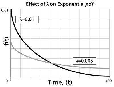
- As [math]\displaystyle{ \lambda \,\! }[/math] is decreased in value, the distribution is stretched out to the right, and as [math]\displaystyle{ \lambda \,\! }[/math] is increased, the distribution is pushed toward the origin.
- This distribution has no shape parameter as it has only one shape, (i.e., the exponential, and the only parameter it has is the failure rate, [math]\displaystyle{ \lambda \,\! }[/math]).
- The distribution starts at [math]\displaystyle{ t=0\,\! }[/math] at the level of [math]\displaystyle{ f(t=0)=\lambda \,\! }[/math] and decreases thereafter exponentially and monotonically as [math]\displaystyle{ t\,\! }[/math] increases, and is convex.
- As [math]\displaystyle{ t\to \infty \,\! }[/math], [math]\displaystyle{ f(t)\to 0\,\! }[/math].
- The pdf can be thought of as a special case of the Weibull pdf with [math]\displaystyle{ \gamma =0\,\! }[/math] and [math]\displaystyle{ \beta =1\,\! }[/math].
Exponential Distribution Functions
The Mean or MTTF
The mean, [math]\displaystyle{ \overline{T},\,\! }[/math] or mean time to failure (MTTF) is given by:
- [math]\displaystyle{ \begin{align} \bar{T}= & \int_{\gamma }^{\infty }t\cdot f(t)dt \\ = & \int_{\gamma }^{\infty }t\cdot \lambda \cdot {{e}^{-\lambda t}}dt \\ = & \gamma +\frac{1}{\lambda }=m \end{align}\,\! }[/math]
Note that when [math]\displaystyle{ \gamma =0\,\! }[/math], the MTTF is the inverse of the exponential distribution's constant failure rate. This is only true for the exponential distribution. Most other distributions do not have a constant failure rate. Consequently, the inverse relationship between failure rate and MTTF does not hold for these other distributions.
The Median
The median, [math]\displaystyle{ \breve{T}, \,\! }[/math] is:
- [math]\displaystyle{ \breve{T}=\gamma +\frac{1}{\lambda}\cdot 0.693 \,\! }[/math]
The Mode
The mode, [math]\displaystyle{ \tilde{T},\,\! }[/math] is:
- [math]\displaystyle{ \tilde{T}=\gamma \,\! }[/math]
The Standard Deviation
The standard deviation, [math]\displaystyle{ {\sigma }_{T}\,\! }[/math], is:
- [math]\displaystyle{ {\sigma}_{T}=\frac{1}{\lambda }=m\,\! }[/math]
The Exponential Reliability Function
The equation for the 2-parameter exponential cumulative density function, or cdf, is given by:
- [math]\displaystyle{ \begin{align} F(t)=Q(t)=1-{{e}^{-\lambda (t-\gamma )}} \end{align}\,\! }[/math]
Recalling that the reliability function of a distribution is simply one minus the cdf, the reliability function of the 2-parameter exponential distribution is given by:
- [math]\displaystyle{ R(t)=1-Q(t)=1-\int_{0}^{t-\gamma }f(x)dx\,\! }[/math]
- [math]\displaystyle{ R(t)=1-\int_{0}^{t-\gamma }\lambda {{e}^{-\lambda x}}dx={{e}^{-\lambda (t-\gamma )}}\,\! }[/math]
The 1-parameter exponential reliability function is given by:
- [math]\displaystyle{ R(t)={{e}^{-\lambda t}}={{e}^{-\tfrac{t}{m}}}\,\! }[/math]
The Exponential Conditional Reliability Function
The exponential conditional reliability equation gives the reliability for a mission of [math]\displaystyle{ t\,\! }[/math] duration, having already successfully accumulated [math]\displaystyle{ T\,\! }[/math] hours of operation up to the start of this new mission. The exponential conditional reliability function is:
- [math]\displaystyle{ R(t|T)=\frac{R(T+t)}{R(T)}=\frac{{{e}^{-\lambda (T+t-\gamma )}}}{{{e}^{-\lambda (T-\gamma )}}}={{e}^{-\lambda t}}\,\! }[/math]
which says that the reliability for a mission of [math]\displaystyle{ t\,\! }[/math] duration undertaken after the component or equipment has already accumulated [math]\displaystyle{ T\,\! }[/math] hours of operation from age zero is only a function of the mission duration, and not a function of the age at the beginning of the mission. This is referred to as the memoryless property.
The Exponential Reliable Life Function
The reliable life, or the mission duration for a desired reliability goal, [math]\displaystyle{ {{t}_{R}}\,\! }[/math], for the 1-parameter exponential distribution is:
- [math]\displaystyle{ R({{t}_{R}})={{e}^{-\lambda ({{t}_{R}}-\gamma )}}\,\! }[/math]
- [math]\displaystyle{ \begin{align} \ln[R({{t}_{R}})]=-\lambda({{t}_{R}}-\gamma ) \end{align}\,\! }[/math]
or:
- [math]\displaystyle{ {{t}_{R}}=\gamma -\frac{\ln [R({{t}_{R}})]}{\lambda }\,\! }[/math]
The Exponential Failure Rate Function
The exponential failure rate function is:
- [math]\displaystyle{ \lambda (t)=\frac{f(t)}{R(t)}=\frac{\lambda {{e}^{-\lambda (t-\gamma )}}}{{{e}^{-\lambda (t-\gamma )}}}=\lambda =\text{constant}\,\! }[/math]
Once again, note that the constant failure rate is a characteristic of the exponential distribution, and special cases of other distributions only. Most other distributions have failure rates that are functions of time.
Characteristics of the Exponential Distribution
The primary trait of the exponential distribution is that it is used for modeling the behavior of items with a constant failure rate. It has a fairly simple mathematical form, which makes it fairly easy to manipulate. Unfortunately, this fact also leads to the use of this model in situations where it is not appropriate. For example, it would not be appropriate to use the exponential distribution to model the reliability of an automobile. The constant failure rate of the exponential distribution would require the assumption that the automobile would be just as likely to experience a breakdown during the first mile as it would during the one-hundred-thousandth mile. Clearly, this is not a valid assumption. However, some inexperienced practitioners of reliability engineering and life data analysis will overlook this fact, lured by the siren-call of the exponential distribution's relatively simple mathematical models.
The Effect of lambda and gamma on the Exponential pdf
- The exponential pdf has no shape parameter, as it has only one shape.
- The exponential pdf is always convex and is stretched to the right as [math]\displaystyle{ \lambda \,\! }[/math] decreases in value.
- The value of the pdf function is always equal to the value of [math]\displaystyle{ \lambda \,\! }[/math] at [math]\displaystyle{ t=0\,\! }[/math] (or [math]\displaystyle{ t=\gamma \,\! }[/math]).
- The location parameter, [math]\displaystyle{ \gamma \,\! }[/math], if positive, shifts the beginning of the distribution by a distance of [math]\displaystyle{ \gamma \,\! }[/math] to the right of the origin, signifying that the chance failures start to occur only after [math]\displaystyle{ \gamma \,\! }[/math] hours of operation, and cannot occur before this time.
- The scale parameter is [math]\displaystyle{ \tfrac{1}{\lambda }=\bar{T}-\gamma =m-\gamma \,\! }[/math].
- As [math]\displaystyle{ t\to \infty \,\! }[/math], [math]\displaystyle{ f(t)\to 0\,\! }[/math].
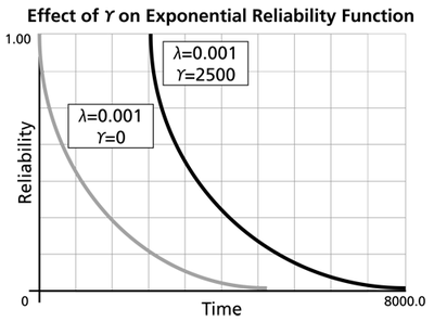
The Effect of lambda and gamma on the Exponential Reliability Function
- The 1-parameter exponential reliability function starts at the value of 100% at [math]\displaystyle{ t=0\,\! }[/math], decreases thereafter monotonically and is convex.
- The 2-parameter exponential reliability function remains at the value of 100% for [math]\displaystyle{ t=0\,\! }[/math] up to [math]\displaystyle{ t=\gamma \,\! }[/math], and decreases thereafter monotonically and is convex.
- As [math]\displaystyle{ t\to \infty \,\! }[/math], [math]\displaystyle{ R(t\to \infty )\to 0\,\! }[/math].
- The reliability for a mission duration of [math]\displaystyle{ t=m=\tfrac{1}{\lambda }\,\! }[/math], or of one MTTF duration, is always equal to [math]\displaystyle{ 0.3679\,\! }[/math] or 36.79%. This means that the reliability for a mission which is as long as one MTTF is relatively low and is not recommended because only 36.8% of the missions will be completed successfully. In other words, of the equipment undertaking such a mission, only 36.8% will survive their mission.
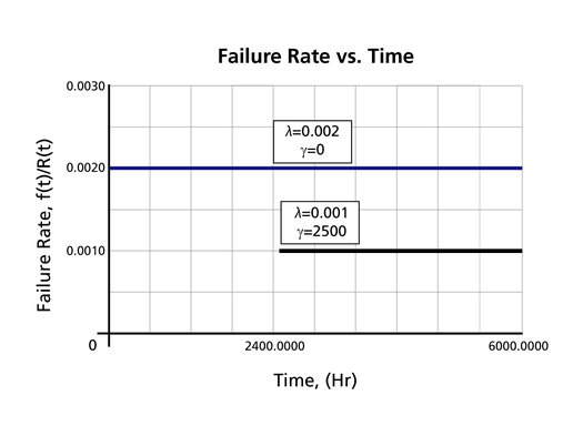
The Effect of lambda and gamma on the Failure Rate Function
- The 1-parameter exponential failure rate function is constant and starts at [math]\displaystyle{ t=0\,\! }[/math].
- The 2-parameter exponential failure rate function remains at the value of 0 for [math]\displaystyle{ t=0\,\! }[/math] up to [math]\displaystyle{ t=\gamma \,\! }[/math], and then keeps at the constant value of [math]\displaystyle{ \lambda\,\! }[/math].
Exponential Distribution Examples
Grouped Data
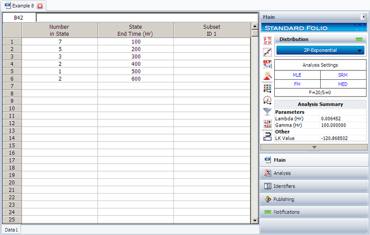
20 units were reliability tested with the following results:
| Table - Life Test Data | |
| Number of Units in Group | Time-to-Failure |
|---|---|
| 7 | 100 |
| 5 | 200 |
| 3 | 300 |
| 2 | 400 |
| 1 | 500 |
| 2 | 600 |
1. Assuming a 2-parameter exponential distribution, estimate the parameters by hand using the MLE analysis method.
2. Repeat the above using Weibull++. (Enter the data as grouped data to duplicate the results.)
3. Show the Probability plot for the analysis results.
4. Show the Reliability vs. Time plot for the results.
5. Show the pdf plot for the results.
6. Show the Failure Rate vs. Time plot for the results.
7. Estimate the parameters using the rank regression on Y (RRY) analysis method (and using grouped ranks).
Solution
1. For the 2-parameter exponential distribution and for [math]\displaystyle{ \hat{\gamma }=100\,\! }[/math] hours (first failure), the partial of the log-likelihood function, [math]\displaystyle{ \lambda\,\! }[/math], becomes:
- [math]\displaystyle{ \begin{align} \frac{\partial \Lambda }{\partial \lambda }= &\underset{i=1}{\overset{6}{\mathop \sum }}\,{N_i} \left[ \frac{1}{\lambda }-\left( {{T}_{i}}-100 \right) \right]=0\\ \Rightarrow & 7[\frac{1}{\lambda }-(100-100)]+5[\frac{1}{\lambda}-(200-100)] + \ldots +2[\frac{1}{\lambda}-(600-100)]\\ = & 0\\ \Rightarrow & \hat{\lambda}=\frac{20}{3100}=0.0065 \text{fr/hr} \end{align} \,\! }[/math]
2. Enter the data in a Weibull++ standard folio and calculate it as shown next.
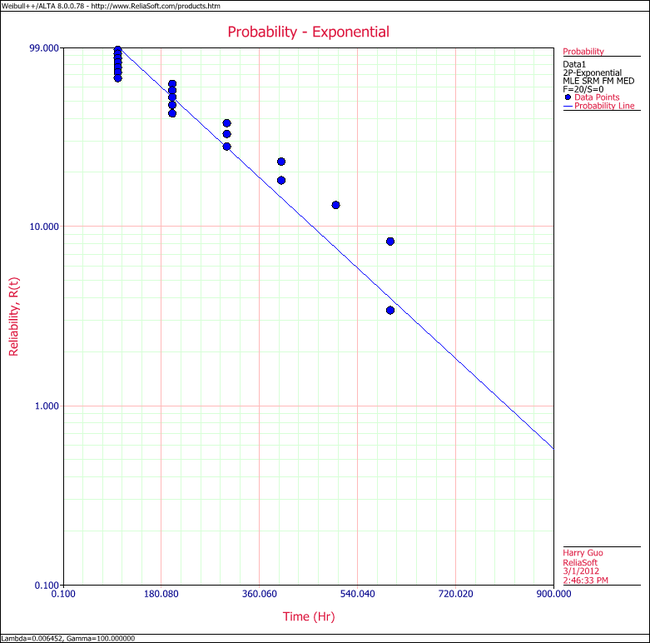
3. On the Plot page of the folio, the exponential Probability plot will appear as shown next.
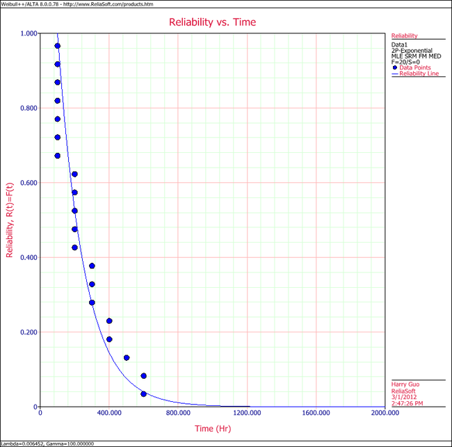
4. View the Reliability vs. Time plot.
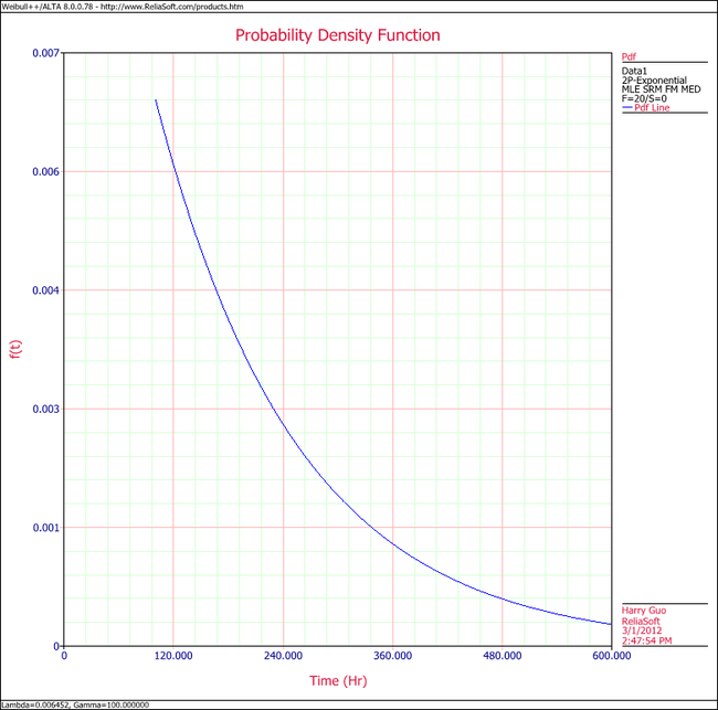
5. View the pdf plot.
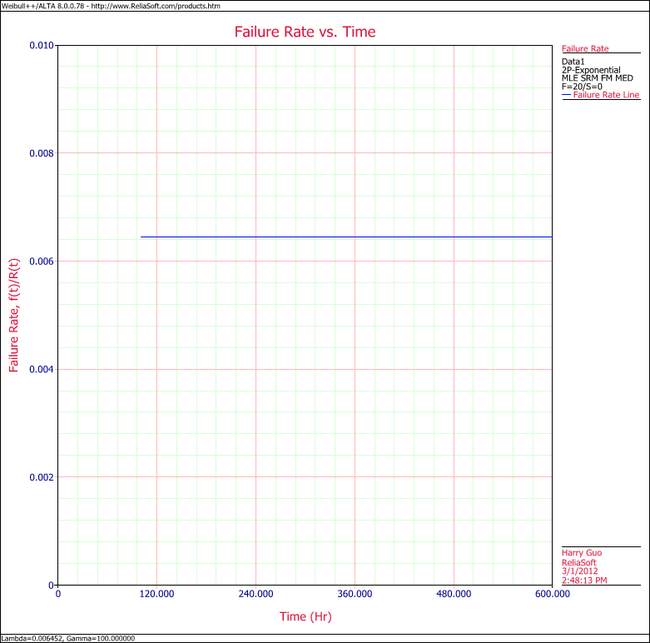
6. View the Failure Rate vs. Time plot.
Note that, as described at the beginning of this chapter, the failure rate for the exponential distribution is constant. Also note that the Failure Rate vs. Time plot does show values for times before the location parameter, [math]\displaystyle{ \gamma \,\! }[/math], at 100 hours.
7. In the case of grouped data, one must be cautious when estimating the parameters using a rank regression method. This is because the median rank values are determined from the total number of failures observed by time [math]\displaystyle{ {{T}_{i}}\,\! }[/math] where [math]\displaystyle{ i\,\! }[/math] indicates the group number. In this example, the total number of groups is [math]\displaystyle{ N=6\,\! }[/math] and the total number of units is [math]\displaystyle{ {{N}_{T}}=20\,\! }[/math]. Thus, the median rank values will be estimated for 20 units and for the total failed units ([math]\displaystyle{ {{N}_{{{F}_{i}}}}\,\! }[/math]) up to the [math]\displaystyle{ {{i}^{th}}\,\! }[/math] group, for the [math]\displaystyle{ {{i}^{th}}\,\! }[/math] rank value. The median ranks values can be found from rank tables or they can be estimated using ReliaSoft's Quick Statistical Reference tool.
For example, the median rank value of the fourth group will be the [math]\displaystyle{ {{17}^{th}}\,\! }[/math] rank out of a sample size of twenty units (or 81.945%).
The following table is then constructed.
Given the values in the table above, calculate [math]\displaystyle{ \hat{a}\,\! }[/math] and [math]\displaystyle{ \hat{b}\,\! }[/math]:
- [math]\displaystyle{ \begin{align} & \hat{b}= & \frac{\underset{i=1}{\overset{6}{\mathop{\sum }}}\,{{t}_{i}}{{y}_{i}}-(\underset{i=1}{\overset{6}{\mathop{\sum }}}\,{{t}_{i}})(\underset{i=1}{\overset{6}{\mathop{\sum }}}\,{{y}_{i}})/6}{\underset{i=1}{\overset{6}{\mathop{\sum }}}\,t_{i}^{2}-{{(\underset{i=1}{\overset{6}{\mathop{\sum }}}\,{{t}_{i}})}^{2}}/6} \\ & & \\ & \hat{b}= & \frac{-4320.3362-(2100)(-9.6476)/6}{910,000-{{(2100)}^{2}}/6} \end{align}\,\! }[/math]
or:
- [math]\displaystyle{ \hat{b}=-0.005392\,\! }[/math]
and:
- [math]\displaystyle{ \hat{a}=\overline{y}-\hat{b}\overline{t}=\frac{\underset{i=1}{\overset{N}{\mathop{\sum }}}\,{{y}_{i}}}{N}-\hat{b}\frac{\underset{i=1}{\overset{N}{\mathop{\sum }}}\,{{t}_{i}}}{N}\,\! }[/math]
or:
- [math]\displaystyle{ \hat{a}=\frac{-9.6476}{6}-(-0.005392)\frac{2100}{6}=0.2793\,\! }[/math]
Therefore:
- [math]\displaystyle{ \hat{\lambda }=-\hat{b}=-(-0.005392)=0.05392\text{ failures/hour}\,\! }[/math]
and:
- [math]\displaystyle{ \hat{\gamma }=\frac{\hat{a}}{\hat{\lambda }}=\frac{0.2793}{0.005392}\,\! }[/math]
or:
- [math]\displaystyle{ \hat{\gamma }\simeq 51.8\text{ hours}\,\! }[/math]
Then:
- [math]\displaystyle{ f(T)=(0.005392){{e}^{-0.005392(T-51.8)}}\,\! }[/math]
Using Weibull++, the estimated parameters are:
- [math]\displaystyle{ \begin{align} \hat{\lambda }= & 0.0054\text{ failures/hour} \\ \hat{\gamma }= & 51.82\text{ hours} \end{align}\,\! }[/math]
The small difference in the values from Weibull++ is due to rounding. In the application, the calculations and the rank values are carried out up to the [math]\displaystyle{ 15^{th}\,\! }[/math] decimal point.
Using Auto Batch Run
A number of leukemia patients were treated with either drug 6MP or a placebo, and the times in weeks until cancer symptoms returned were recorded. Analyze each treatment separately [21, p.175].
| Table - Leukemia Treatment Results | |||
| Time (weeks) | Number of Patients | Treament | Comments |
|---|---|---|---|
| 1 | 2 | placebo | |
| 2 | 2 | placebo | |
| 3 | 1 | placebo | |
| 4 | 2 | placebo | |
| 5 | 2 | placebo | |
| 6 | 4 | 6MP | 3 patients completed |
| 7 | 1 | 6MP | |
| 8 | 4 | placebo | |
| 9 | 1 | 6MP | Not completed |
| 10 | 2 | 6MP | 1 patient completed |
| 11 | 2 | placebo | |
| 11 | 1 | 6MP | Not completed |
| 12 | 2 | placebo | |
| 13 | 1 | 6MP | |
| 15 | 1 | placebo | |
| 16 | 1 | 6MP | |
| 17 | 1 | placebo | |
| 17 | 1 | 6MP | Not completed |
| 19 | 1 | 6MP | Not completed |
| 20 | 1 | 6MP | Not completed |
| 22 | 1 | placebo | |
| 22 | 1 | 6MP | |
| 23 | 1 | placebo | |
| 23 | 1 | 6MP | |
| 25 | 1 | 6MP | Not completed |
| 32 | 2 | 6MP | Not completed |
| 34 | 1 | 6MP | Not completed |
| 35 | 1 | 6MP | Not completed |
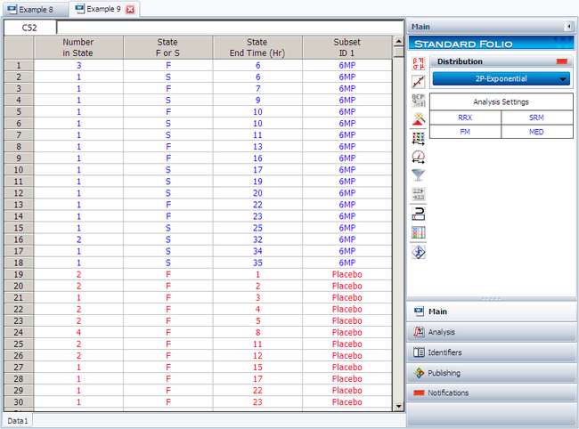
Create a new Weibull++ standard folio that's configured for grouped times-to-failure data with suspensions. In the first column, enter the number of patients. Whenever there are uncompleted tests, enter the number of patients who completed the test separately from the number of patients who did not (e.g., if 4 patients had symptoms return after 6 weeks and only 3 of them completed the test, then enter 1 in one row and 3 in another). In the second column enter F if the patients completed the test and S if they didn't. In the third column enter the time, and in the fourth column (Subset ID) specify whether the 6MP drug or a placebo was used.
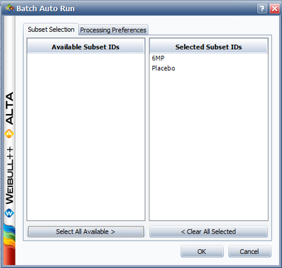
Next, open the Batch Auto Run utility and select to separate the 6MP drug from the placebo, as shown next.
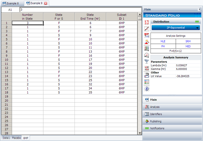
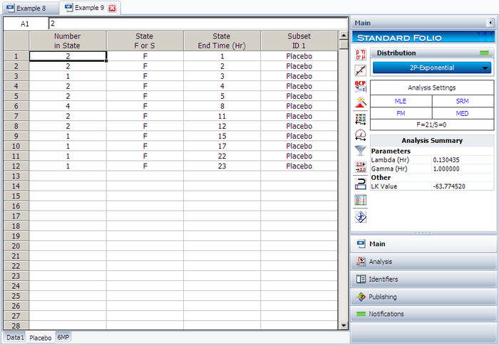
The software will create two data sheets, one for each subset ID, as shown next.
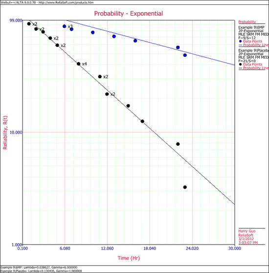
Calculate both data sheets using the 2-parameter exponential distribution and the MLE analysis method, then insert an additional plot and select to show the analysis results for both data sheets on that plot, which will appear as shown next.
Bayesian Non-Parametric Test Design
The regular non-parametric analyses performed based on either the binomial or the chi-squared equation were performed with only the direct system test data. However, if prior information regarding system performance is available, it can be incorporated into a Bayesian non-parametric analysis. This subsection will demonstrate how to incorporate prior information about system reliability and also how to incorporate prior information from subsystem tests into system test design.
Assumption on System Reliability
If we assume the system reliability follows a beta distribution, the values of system reliability, R, confidence level, CL, number of units tested, n, and number of failures, r, are related by the following equation:
where [math]\displaystyle{ Beta }[/math] is the incomplete beta function. If α0 and β0 are known, then any quantity of interest can be calculated using the remaining three. The next two examples demonstrate how to calculate α0 and β0 depending on the type of prior information available.
Use Prior Expert Opinion on System Reliability
Prior information on system reliability can be exploited to determine [math]\displaystyle{ \alpha_{0} }[/math] and [math]\displaystyle{ \beta_{0} }[/math]. To do so, first approximate the expected value and variance of prior system reliability R0. This requires knowledge of the lowest possible reliability, the most likely possible reliability and the highest possible reliability of the system. These quantities will be referred to as a, b and c, respectively. The expected value of the prior system reliability is approximately given as:
- [math]\displaystyle{ E\left(R_{0}\right)=\frac{a+4b+c}{6} }[/math]
and the variance is approximately given by:
- [math]\displaystyle{ Var\left(R_{0}\right)=\frac{c-a}{6} }[/math]
These approximate values of the expected value and variance of the prior system reliability can then be used to estimate the values of [math]\displaystyle{ \alpha_{0} }[/math] and [math]\displaystyle{ \beta_{0} }[/math], assuming that the prior reliability is a beta-distributed random variable. The values of [math]\displaystyle{ \alpha_{0} }[/math] and [math]\displaystyle{ \beta_{0} }[/math] are calculated as:
With [math]\displaystyle{ \alpha_{0} }[/math] and [math]\displaystyle{ \beta_{0} }[/math] known, the above beta distribution equation can now be used to calculate a quantity of interest.
Example 3:
You can use the non-parametric Bayesian method to design a test using prior knowledge about a system's reliability. For example, suppose you wanted to know the reliability of a system and you had the following prior knowledge of the system:
- Lowest possible reliability: a = 0.8
- Most likely reliability: b = 0.85
- Highest possible reliability: c = 0.97
This information can be used to approximate the expected value and the variance of the prior system reliability.
- [math]\displaystyle{ E\left(R_{0}\right)=\frac{a+4b+c}{6}=0.861667 \,\! }[/math]
- [math]\displaystyle{ Var({{R}_{0}})={{\left( \frac{c-a}{6} \right)}^{2}}=0.000803 \,\! }[/math]
These approximations of the expected value and variance of the prior system reliability can then be used to estimate [math]\displaystyle{ \alpha_{0}\,\! }[/math] and [math]\displaystyle{ \beta_{0}\,\! }[/math] used in the beta distribution for the system reliability, as given next:
- [math]\displaystyle{ \alpha\,\!_{0}=E\left(R_{0}\right)\left[\frac{E\left(R_{0}\right)-E^{2}\left(R_{0}\right)}{Var\left(R_{0}\right)}-1\right]=127.0794\,\! }[/math]
- [math]\displaystyle{ \beta\,\!_{0}=\left(1-E\left(R_{0}\right)\right)\left[\frac{E\left(R_{0}\right)-E^{2}\left(R_{0}\right)}{Var\left(R_{0}\right)}-1\right]=20.40153\,\! }[/math]
With [math]\displaystyle{ \alpha_{0}\,\! }[/math] and [math]\displaystyle{ \beta_{0}\,\! }[/math] known, any single value of the four quantities system reliability R, confidence level CL, number of units n, or number of failures r can be calculated from the other three using the beta distribution function:
- [math]\displaystyle{ 1-CL=\text{Beta}\left(R,\alpha,\beta\right)=\text{Beta}\left(R,n-r+\alpha_{0},r+\beta_{0}\right)\,\! }[/math]
Solve for System Reliability R
Given CL = 0.9, n = 20, and r = 1, using the above prior information to solve R.
First, we get the number of successes: s = n – r = 19. Then the parameters in the posterior beta distribution for R are calculated as:
- [math]\displaystyle{ \alpha\,\!=\alpha\,\!_{0}+s=146.0794\,\! }[/math]
- [math]\displaystyle{ \beta\,\!=\beta\,\!_{0}+r=21.40153\,\! }[/math]
Finally, from this posterior distribution, the system reliability R at a confidence level of CL=0.9 is solved as:
- [math]\displaystyle{ R=\text{BetaINV}\left(1-CL,\alpha\,\!,\beta\,\!\right)=0.838374 \,\! }[/math]
Solve for Confidence Level CL
Given R = 0.85, n = 20, and r = 1, using the above prior information on system reliability to solve for CL.
First, we get the number of successes: s = n – r = 19. Then the parameters in the posterior beta distribution for R are calculated as:
- [math]\displaystyle{ \alpha\,\!=\alpha\,\!_{0}+s=146.07943\,\! }[/math]
- [math]\displaystyle{ \beta\,\!=\beta\,\!_{0}+r=21.40153\,\! }[/math]
Finally, from this posterior distribution, the corresponding confidence level for reliability R=0.85 is:
- [math]\displaystyle{ CL=\text{Beta}\left(R,\alpha,\beta\right)=0.81011 \,\! }[/math]
Solve for Sample Size n
Given R = 0.9, CL = 0.8, and r = 1, using the above prior information on system reliability to solve the required sample size in the demonstration test.
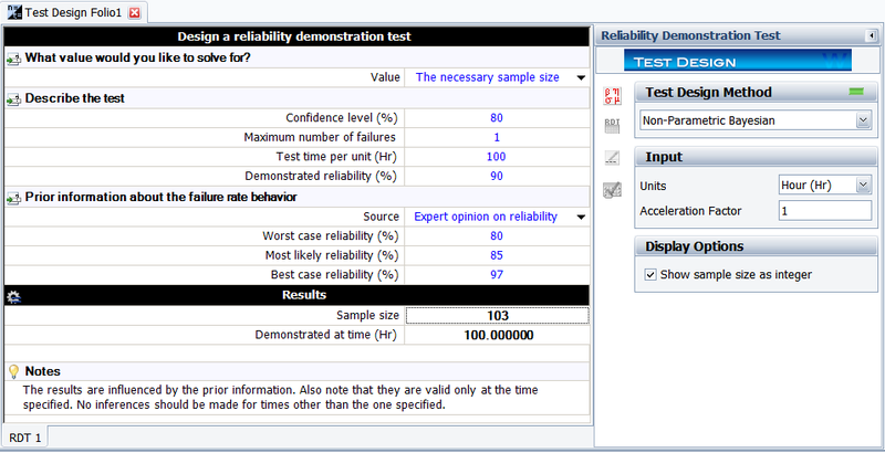
Again, the above beta distribution equation for the system reliability can be utilized. The figure below shows the result from Weibull++. The results show that the required sample size is 103. Weibull++ always displays the sample size as an integer.
Use Prior Information from Subsystem Tests
Prior information from subsystem tests can also be used to determine values of alpha and beta. Information from subsystem tests can be used to calculate the expected value and variance of the reliability of individual components, which can then be used to calculate the expected value and variance of the reliability of the entire system. [math]\displaystyle{ \alpha_{0} }[/math] and [math]\displaystyle{ \beta_{0} }[/math] are then calculated as before:
For each subsystem i, from the beta distribution, we can calculate the expected value and the variance of the subsystem’s reliability [math]\displaystyle{ R_{i} }[/math] as [38]:
Assuming that all the subsystems are in a series reliability-wise configuration, the expected value and variance of the system’s reliability [math]\displaystyle{ R }[/math] can then be calculated as [38]:
With the above prior information on the expected value and variance of the system reliability, all the calculations can now be calculated as before.
Example 5:
Template:Example: Bayesian Test Design with Prior Information from Subsystem Tests
Test Design Using Expected Failure Time Plots
Test duration is one of the key factors that should be considered in designing a test. If the expected test duration can be estimated prior to the test, test resources can be better allocated. In this section, we will explain how to estimate the expected test time based on test sample size and the assumed underlying failure distribution.
The binomial equation used in non-parametric demonstration test design is the base for predicting expected failure times. The equation is:
where:
- [math]\displaystyle{ \begin{align} & CL= \text{the required confidence level} \\ & r= \text{the number of failures} \\ & n= \text{the total number of units on test} \\ & {{R}_{TEST}}= \text{the reliability on test} \end{align} }[/math]
If CL, r and n are given, the R value can be solved from the above equation. When CL=0.5, the solved R (or Q, the probability of failure whose value is 1-R) is the so called median rank for the corresponding failure. Please see Median Ranks.
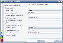
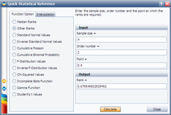
For example, given n = 4, r = 2 and CL = 0.5, the calculated Q is 0.385728. This means, at the time when the second failure occurs, the estimated system probability of failure is 0.385728. The median rank can be calculated in Weibull++ using the Quick Statistical Reference, as shown below:
Similarly, if we set r = 3 for the above example, we can get the probability of failure at the time when the third failure occurs. Using the estimated median rank for each failure and the assumed underlying failure distribution, we can calculate the expected time for each failure. Assume the failure distribution is Weibull, then we know:
where:
- [math]\displaystyle{ \beta }[/math] is the shape parameter
- [math]\displaystyle{ \eta }[/math] is the scale parameter
Using the above equation, for a given Q, we can get the corresponding time t. The above calculation gives the median of each failure time for CL = 0.5. If we set CL at different values, the confidence bounds of each failure time can be obtained. For the above example, if we set CL=0.9, from the calculated Q we can get the upper bound of the time for each failure. The calculated Q is given in the next figure:
If we set CL=0.1, from the calculated Q we can get the lower bound of the time for each failure. The calculated Q is given in the figure below:
Example 6:
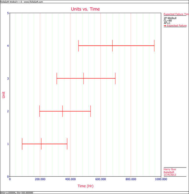
In this example you will use the Expected Failure Times plot to estimate the duration of a planned reliability test. 4 units were allocated for the test, and the test engineers want to know how long the test will last if all the units are tested to failure. Based on previous experiments, they assume the underlying failure distribution is a Weibull distribution with [math]\displaystyle{ \beta = 2\,\! }[/math] and [math]\displaystyle{ \eta = 500\,\! }[/math].
Solution
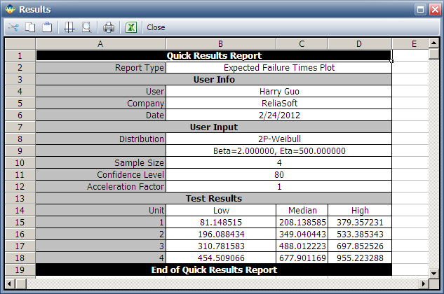
Using Weibull++'s Expected Failure Times plot, the expected failure times with 80% 2-sided confidence bounds are given below.
From the above results, we can see the upper bound of the last failure is about 955 hours. Therefore, the test probably will last for around 955 hours.
As we know, with 4 samples, the median rank for the second failure is 0.385728. Using this value and the assumed Weibull distribution, the median value of the failure time of the second failure is calculated as:
- [math]\displaystyle{ \begin{align} & Q=1-{{e}^-{{{\left( \frac{t}{\eta } \right)}^{\beta }}}}\Rightarrow \\ & \ln (1-Q)={{\left( \frac{t}{\eta } \right)}^{\beta }} \\ & \Rightarrow t=\text{349.04}\\ \end{align}\,\! }[/math]
Its bounds and other failure times can be calculated in a similar way.
Test Design Using a Life Difference Detection Matrix
Engineers often need to design tests for detecting life differences between two or more product designs. The questions are how many samples and how long should the test be conducted in order to detect a certain amount of difference. There are no simple answers. Usually, advanced design of experiments (DOE) techniques should be utilized. For a simple case, such as comparing two designs, the Difference Detection Matrix in Weibull++ can be used. The difference detection matrix graphically indicates the amount of test time required to detect a statistical difference in the lives of two populations.
As discussed in the test design using expected failure times plot, if the sample size is known, the expected failure time of each test unit can be obtained based on the assumed failure distribution. Now let's go one step further. With these failure times, we can then estimate the failure distribution and calculate any reliability metrics. This process is similar to the simulation used in Simumatic where random failure times are generated from simulation and then used to estimate the failure distribution. This approach is also used by the difference detection matrix.
Assume we want to compare the B10 lifes (or mean lifes) of two designs. The test is time-terminated and the termination time is set to T. Using the method given in Test Design Using Expected Failure Time Plots, we can generate the failure times. For any failure time greater than T, it is a suspension and the suspension time is T. For each design, its B10 life and confidence bounds can be estimated from the generated failure/suspension times. If the two estimated confidence intervals overlap with each other, it means the difference of the two B10 lifes cannot be detected from this test. We have to either increase the sample size or the test duration.
Example 7:
In this example, you will use the Difference Detection Matrix to choose the suitable sample size and duration for a reliability test. Assume that there are two design options for a new product. The engineers need to design a test that compares the reliability performance of these two options. The reliability for both designs is assumed to follow a Weibull distribution. For Design 1, its shape parameter [math]\displaystyle{ \beta = 3\,\! }[/math]; for Design 2, its [math]\displaystyle{ \beta= 2\,\! }[/math]. Their B10 lives may range from 500 to 3,000 hours.
Solution
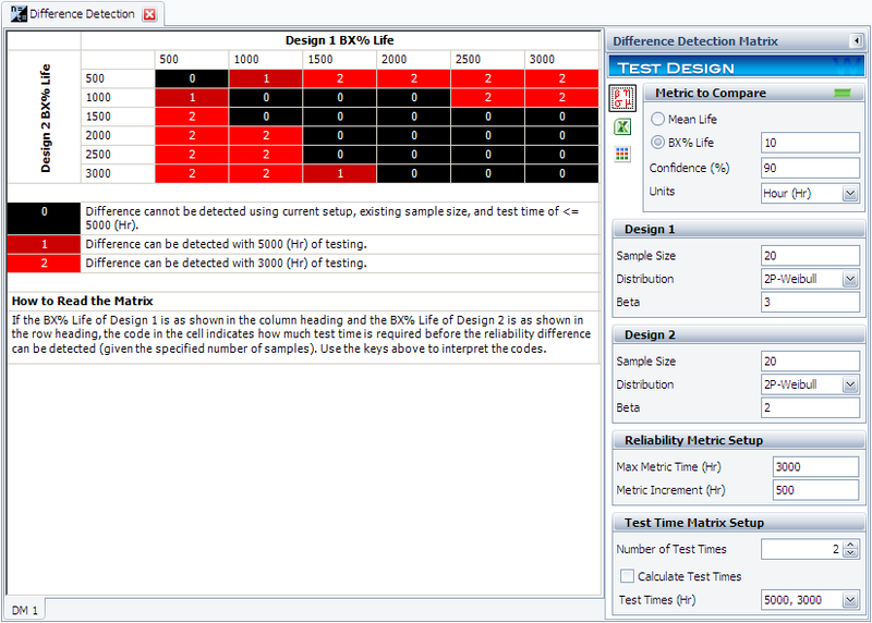
For the initial setup, set the sample size for each design to 20, and use two test durations of 3,000 and 5,000 hours. The following picture shows the complete control panel setup and the results of the analysis.
The columns in the matrix show the range of the assumed B10 life for design 1, while the rows show the range for design 2. A value of 0 means the difference cannot be detected through the test, 1 means the difference can be detected if the test duration is 5,000 hours, and 2 means the difference can be detected if the test duration is 3,000 hours. For example, the number is 2 for cell (1000, 2000). This means that if the B10 life for Design 1 is 1,000 hours and the B10 life for Design 2 is 2,000 hours, the difference can be detected if the test duration is at least 5,000 hours.
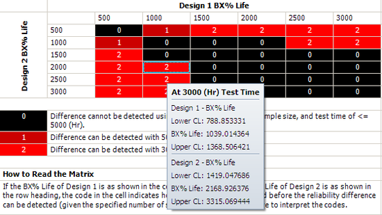
Click inside the cell to show the estimated confidence intervals, as shown next. By testing 20 samples each for 3,000 hours, the difference of their B10 lives probably can be detected. This is because, at a confidence level of 90%, the estimated confidence intervals on the B10 life do not overlap.
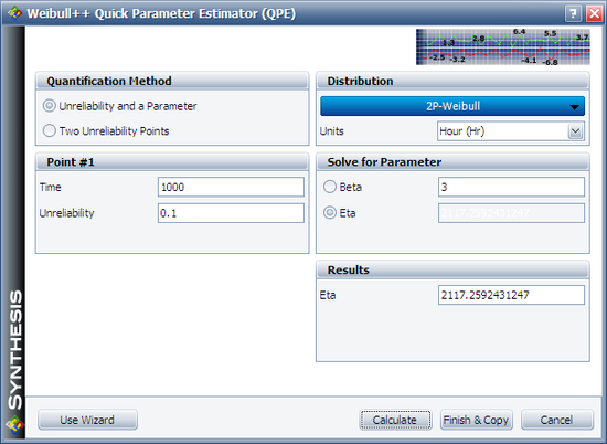
We will use Design 1 to illustrate how the interval is calculated. For cell (1000, 2000), Design 1's B10 life is 1,000 and the assumed [math]\displaystyle{ \beta\,\! }[/math] is 3. We can calculate the [math]\displaystyle{ \eta\,\! }[/math] for the Weibull distribution using the Quick Parameter Estimator tool, as shown next.
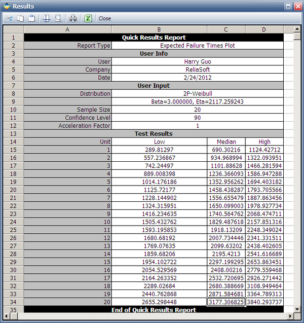
The estimated [math]\displaystyle{ \eta\,\! }[/math] is 2117.2592 hours. We can then use these distribution parameters and the sample size of 20 to get the expected failure times by using Weibull's Expected Failure Times Plot. The following report shows the result from that utility.
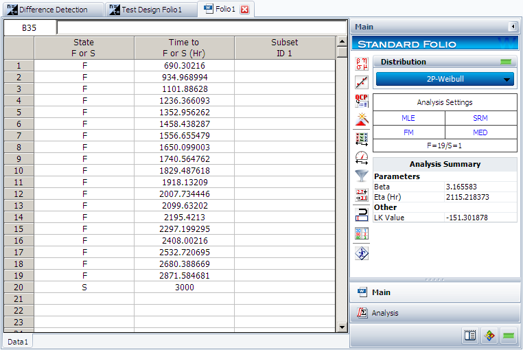
The median failure times are used to estimate the failure distribution. Note that since the test duration is set to 3,000 hours, any failures that occur after 3,000 are treated as suspensions. In this case, the last failure is a suspension with a suspension time of 3,000 hours. We can enter the median failure times data set into a standard Weibull++ folio as given in the next figure.
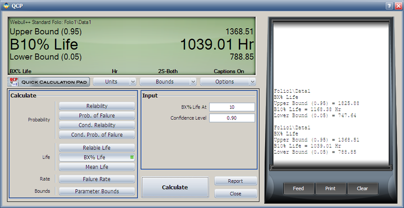
After analyzing the data set with the MLE and FM analysis options, we can now calculate the B10 life and its interval in the QCP, as shown next.
From this result, we can see that the estimated B10 life and its confidence intervals are the same as the results displayed in the Difference Detection Matrix.
The above procedure can be repeated to get the results for the other cells and for Design 2. Therefore, by adjusting the sample size and test duration, a suitable test time can be identified for detecting a certain amount of difference between two designs/populations.
Example 2:
Quite often, there is a desire to design reliability demonstration tests that have few or no failures. These tests are often required to demonstrate customer reliability and confidence requirements. While it is desirable to be able to test a large population of units to failure in order to obtain information on a design's reliability, time and resource constraints sometimes make this impossible. In these cases, a test can be run on a specified number of units for a specified amount of time that will demonstrate that the product has met or exceeded a given reliability at a given confidence level. In order to do so without a large amount of cumulative test time or failure data, it is necessary to make assumptions about the failure distribution of the product. In the final analysis, the actual reliability of the units will, of course, remain unknown, but the reliability engineer will be able to state that certain specifications have been met.
Demonstration Test Design
Frequently, a manufacturer will have to demonstrate that a certain product has met a goal of a certain reliability at a given time with a specific confidence. Often, it will be desired to demonstrate that this goal has been met with a zero-failure test. In order to design and conduct such a test, something about the failure behavior of the product will need to be known (i.e., the shape parameter of the product's life distribution). Beyond this, nothing more about the test is known, and usually the engineer designing the test will have to study the financial trade-offs between the number of units and the amount of test time needed to demonstrate the desired goal. In cases like this, it is useful to have a "carpet plot" that shows the possibilities of how a certain specification can be met.
This methodology requires the use of the cumulative binomial distribution in addition to the assumed distribution of the product's lifetimes. Not only does the life distribution of the product need to be assumed beforehand, but a reasonable assumption of the distribution's shape parameter must be provided as well. Additional information that must be supplied includes: a) the reliability to be demonstrated, b) the confidence level at which the demonstration takes place, c) the acceptable number of failures and d) either the number of available units or the amount of available test time. The output of this analysis can be the amount of time required to test the available units or the required number of units that need to be tested during the available test time.
Reliability Demonstration
Frequently, the entire purpose of designing a test with few or no failures is to demonstrate a certain reliability, [math]\displaystyle{ {{R}_{DEMO}} }[/math], at a certain time. With the exception of the exponential distribution (and ignoring the location parameter for the time being), this reliability is going to be a function of time, a shape parameter and a scale parameter.
where:
- [math]\displaystyle{ {{t}_{DEMO}} }[/math] is the time at which the demonstrated reliability is specified.
- [math]\displaystyle{ \theta }[/math] is the shape parameter.
- [math]\displaystyle{ \phi }[/math] is the scale parameter.
Since required inputs to the process include [math]\displaystyle{ {{R}_{DEMO}} }[/math], [math]\displaystyle{ {{t}_{DEMO}} }[/math] and [math]\displaystyle{ \theta }[/math], the value of the scale parameter can be backed out of the reliability equation of the assumed distribution, and will be used in the calculation of another reliability value, [math]\displaystyle{ {{R}_{TEST}} }[/math], which is the reliability that is going to be incorporated into the actual test calculation. How this calculation is performed depends on whether one is attempting to solve for the number of units to be tested in an available amount of time, or attempting to determine how long to test an available number of test units.
Determining Units for Available Test Time
If one knows that the test is to last a certain amount of time, [math]\displaystyle{ {{t}_{TEST}} }[/math], the number of units that must be tested to demonstrate the specification must be determined. The first step in accomplishing this involves calculating the [math]\displaystyle{ {{R}_{TEST}} }[/math] value.
This should be a simple procedure since:
and [math]\displaystyle{ {{t}_{DEMO}} }[/math], [math]\displaystyle{ \theta }[/math] and [math]\displaystyle{ \phi }[/math] are already known, and it is just a matter of plugging these values into the appropriate reliability equation.
We now incorporate a form of the cumulative binomial distribution in order to solve for the required number of units. This form of the cumulative binomial appears as:
where:
- [math]\displaystyle{ \begin{align} & CL= \text{the required confidence level} \\ & f= \text{the allowable number of failures} \\ & n= \text{the total number of units on test} \\ & {{R}_{TEST}}= \text{the reliability on test} \end{align} }[/math]
Since [math]\displaystyle{ CL }[/math] and [math]\displaystyle{ f }[/math] are required inputs to the process and [math]\displaystyle{ {{R}_{TEST}} }[/math] has already been calculated, it merely remains to solve the cumulative binomial equation for [math]\displaystyle{ n }[/math], the number of units that need to be tested.
Determining Test Time for Available Units
The way that one determines the test time for the available number of test units is quite similar to the process described previously. In this case, one knows beforehand the number of units, [math]\displaystyle{ n }[/math], the number of allowable failures, [math]\displaystyle{ f }[/math], and the confidence level, [math]\displaystyle{ CL }[/math]. With this information, the next step involves solving the binomial equation for [math]\displaystyle{ {{R}_{TEST}} }[/math]. With this value known, one can use the appropriate reliability equation to back out the value of [math]\displaystyle{ {{t}_{TEST}} }[/math], since [math]\displaystyle{ {{R}_{TEST}}=g({{t}_{TEST}};\theta ,\phi ) }[/math], and [math]\displaystyle{ {{R}_{TEST}} }[/math], [math]\displaystyle{ \theta }[/math] and [math]\displaystyle{ \phi }[/math] have already been calculated or specified.
MTTF Demonstration
Designing a test to demonstrate a certain value of the [math]\displaystyle{ MTTF }[/math] is identical to designing a reliability demonstration test, with the exception of how the value of the scale parameter [math]\displaystyle{ \phi }[/math] is determined. Given the value of the [math]\displaystyle{ MTTF }[/math] and the value of the shape parameter [math]\displaystyle{ \theta }[/math] , the value of the scale parameter [math]\displaystyle{ \phi }[/math] can be calculated. With this, the analysis can proceed as with the reliability demonstration methodology.
Non-Parametric Test Design
The binomial equation can be used for nonparametric demonstration test design. One must merely assume values for three of the inputs of [math]\displaystyle{ CL }[/math], [math]\displaystyle{ {{R}_{TEST}} }[/math], [math]\displaystyle{ n }[/math], and [math]\displaystyle{ f }[/math], and solve for the fourth. Note that there is no time value associated with this methodology, so one must assume that the value of [math]\displaystyle{ {{R}_{TEST}} }[/math] is associated with the amount of time for which the units were tested.
Example 1:
Template loop detected: Template:Example: Weibull Distribution Example-Demonstrate Reliability
Example 2:
Template loop detected: Template:Example: Weibull Distribution Example-Demonstrate MTTF
Constant Failure Rate/Chi-Squared Test Design
Another method for designing tests for products that have an assumed constant failure rate, or exponential life distribution, draws on the chi-squared distribution. These represent the true exponential distribution confidence bounds referred to in The Exponential Distribution. This method only returns the necessary accumulated test time for a demonstrated reliability or [math]\displaystyle{ MTTF }[/math] , not a specific time/test unit combination that is obtained using the cumulative binomial method described above. The accumulated test time is equal to the total amount of time experienced by all of the units on test. Assuming that the units undergo the same amount of test time, this works out to be:
where [math]\displaystyle{ n }[/math] is the number of units on test and [math]\displaystyle{ {{t}_{TEST}} }[/math] is the test time. The chi-squared equation for test time is:
where:
- [math]\displaystyle{ \begin{align} & \chi _{1-CL;2f+2}^{2}= \text{the chi squared distribution} \\ & {{T}_{a}}= \text{the necessary accumulated test time} \\ & CL= \text{the confidence level} \\ & f=\text{the number of failures} \end{align} }[/math]
Since this methodology only applies to the exponential distribution, the exponential reliability equation can be rewritten as:
and substituted into the chi-squared equation for developing a test that demonstrates reliability at a given time, rather than [math]\displaystyle{ MTTF }[/math] :
Example 3:
The exponential distribution is a commonly used distribution in reliability engineering. Mathematically, it is a fairly simple distribution, which many times leads to its use in inappropriate situations. It is, in fact, a special case of the Weibull distribution where [math]\displaystyle{ \beta =1\,\! }[/math]. The exponential distribution is used to model the behavior of units that have a constant failure rate (or units that do not degrade with time or wear out).
Exponential Probability Density Function
The 2-Parameter Exponential Distribution
The 2-parameter exponential pdf is given by:
- [math]\displaystyle{ f(t)=\lambda {{e}^{-\lambda (t-\gamma )}},f(t)\ge 0,\lambda \gt 0,t\ge \gamma \,\! }[/math]
where [math]\displaystyle{ \gamma \,\! }[/math] is the location parameter. Some of the characteristics of the 2-parameter exponential distribution are discussed in Kececioglu [19]:
- The location parameter, [math]\displaystyle{ \gamma \,\! }[/math], if positive, shifts the beginning of the distribution by a distance of [math]\displaystyle{ \gamma \,\! }[/math] to the right of the origin, signifying that the chance failures start to occur only after [math]\displaystyle{ \gamma \,\! }[/math] hours of operation, and cannot occur before.
- The scale parameter is [math]\displaystyle{ \tfrac{1}{\lambda }=\bar{t}-\gamma =m-\gamma \,\! }[/math].
- The exponential pdf has no shape parameter, as it has only one shape.
- The distribution starts at [math]\displaystyle{ t=\gamma \,\! }[/math] at the level of [math]\displaystyle{ f(t=\gamma )=\lambda \,\! }[/math] and decreases thereafter exponentially and monotonically as [math]\displaystyle{ t\,\! }[/math] increases beyond [math]\displaystyle{ \gamma \,\! }[/math] and is convex.
- As [math]\displaystyle{ t\to \infty \,\! }[/math], [math]\displaystyle{ f(t)\to 0\,\! }[/math].
The 1-Parameter Exponential Distribution
The 1-parameter exponential pdf is obtained by setting [math]\displaystyle{ \gamma =0\,\! }[/math], and is given by:
- [math]\displaystyle{ \begin{align}f(t)= & \lambda {{e}^{-\lambda t}}=\frac{1}{m}{{e}^{-\tfrac{1}{m}t}}, & t\ge 0, \lambda \gt 0,m\gt 0 \end{align} \,\! }[/math]
where:
- [math]\displaystyle{ \lambda \,\! }[/math] = constant rate, in failures per unit of measurement, (e.g., failures per hour, per cycle, etc.)
- [math]\displaystyle{ \lambda =\frac{1}{m}\,\! }[/math]
- [math]\displaystyle{ m\,\! }[/math] = mean time between failures, or to failure
- [math]\displaystyle{ t\,\! }[/math] = operating time, life, or age, in hours, cycles, miles, actuations, etc.
This distribution requires the knowledge of only one parameter, [math]\displaystyle{ \lambda \,\! }[/math], for its application. Some of the characteristics of the 1-parameter exponential distribution are discussed in Kececioglu [19]:
- The location parameter, [math]\displaystyle{ \gamma \,\! }[/math], is zero.
- The scale parameter is [math]\displaystyle{ \tfrac{1}{\lambda }=m\,\! }[/math].
- As [math]\displaystyle{ \lambda \,\! }[/math] is decreased in value, the distribution is stretched out to the right, and as [math]\displaystyle{ \lambda \,\! }[/math] is increased, the distribution is pushed toward the origin.
- This distribution has no shape parameter as it has only one shape, (i.e., the exponential, and the only parameter it has is the failure rate, [math]\displaystyle{ \lambda \,\! }[/math]).
- The distribution starts at [math]\displaystyle{ t=0\,\! }[/math] at the level of [math]\displaystyle{ f(t=0)=\lambda \,\! }[/math] and decreases thereafter exponentially and monotonically as [math]\displaystyle{ t\,\! }[/math] increases, and is convex.
- As [math]\displaystyle{ t\to \infty \,\! }[/math], [math]\displaystyle{ f(t)\to 0\,\! }[/math].
- The pdf can be thought of as a special case of the Weibull pdf with [math]\displaystyle{ \gamma =0\,\! }[/math] and [math]\displaystyle{ \beta =1\,\! }[/math].
Exponential Distribution Functions
The Mean or MTTF
The mean, [math]\displaystyle{ \overline{T},\,\! }[/math] or mean time to failure (MTTF) is given by:
- [math]\displaystyle{ \begin{align} \bar{T}= & \int_{\gamma }^{\infty }t\cdot f(t)dt \\ = & \int_{\gamma }^{\infty }t\cdot \lambda \cdot {{e}^{-\lambda t}}dt \\ = & \gamma +\frac{1}{\lambda }=m \end{align}\,\! }[/math]
Note that when [math]\displaystyle{ \gamma =0\,\! }[/math], the MTTF is the inverse of the exponential distribution's constant failure rate. This is only true for the exponential distribution. Most other distributions do not have a constant failure rate. Consequently, the inverse relationship between failure rate and MTTF does not hold for these other distributions.
The Median
The median, [math]\displaystyle{ \breve{T}, \,\! }[/math] is:
- [math]\displaystyle{ \breve{T}=\gamma +\frac{1}{\lambda}\cdot 0.693 \,\! }[/math]
The Mode
The mode, [math]\displaystyle{ \tilde{T},\,\! }[/math] is:
- [math]\displaystyle{ \tilde{T}=\gamma \,\! }[/math]
The Standard Deviation
The standard deviation, [math]\displaystyle{ {\sigma }_{T}\,\! }[/math], is:
- [math]\displaystyle{ {\sigma}_{T}=\frac{1}{\lambda }=m\,\! }[/math]
The Exponential Reliability Function
The equation for the 2-parameter exponential cumulative density function, or cdf, is given by:
- [math]\displaystyle{ \begin{align} F(t)=Q(t)=1-{{e}^{-\lambda (t-\gamma )}} \end{align}\,\! }[/math]
Recalling that the reliability function of a distribution is simply one minus the cdf, the reliability function of the 2-parameter exponential distribution is given by:
- [math]\displaystyle{ R(t)=1-Q(t)=1-\int_{0}^{t-\gamma }f(x)dx\,\! }[/math]
- [math]\displaystyle{ R(t)=1-\int_{0}^{t-\gamma }\lambda {{e}^{-\lambda x}}dx={{e}^{-\lambda (t-\gamma )}}\,\! }[/math]
The 1-parameter exponential reliability function is given by:
- [math]\displaystyle{ R(t)={{e}^{-\lambda t}}={{e}^{-\tfrac{t}{m}}}\,\! }[/math]
The Exponential Conditional Reliability Function
The exponential conditional reliability equation gives the reliability for a mission of [math]\displaystyle{ t\,\! }[/math] duration, having already successfully accumulated [math]\displaystyle{ T\,\! }[/math] hours of operation up to the start of this new mission. The exponential conditional reliability function is:
- [math]\displaystyle{ R(t|T)=\frac{R(T+t)}{R(T)}=\frac{{{e}^{-\lambda (T+t-\gamma )}}}{{{e}^{-\lambda (T-\gamma )}}}={{e}^{-\lambda t}}\,\! }[/math]
which says that the reliability for a mission of [math]\displaystyle{ t\,\! }[/math] duration undertaken after the component or equipment has already accumulated [math]\displaystyle{ T\,\! }[/math] hours of operation from age zero is only a function of the mission duration, and not a function of the age at the beginning of the mission. This is referred to as the memoryless property.
The Exponential Reliable Life Function
The reliable life, or the mission duration for a desired reliability goal, [math]\displaystyle{ {{t}_{R}}\,\! }[/math], for the 1-parameter exponential distribution is:
- [math]\displaystyle{ R({{t}_{R}})={{e}^{-\lambda ({{t}_{R}}-\gamma )}}\,\! }[/math]
- [math]\displaystyle{ \begin{align} \ln[R({{t}_{R}})]=-\lambda({{t}_{R}}-\gamma ) \end{align}\,\! }[/math]
or:
- [math]\displaystyle{ {{t}_{R}}=\gamma -\frac{\ln [R({{t}_{R}})]}{\lambda }\,\! }[/math]
The Exponential Failure Rate Function
The exponential failure rate function is:
- [math]\displaystyle{ \lambda (t)=\frac{f(t)}{R(t)}=\frac{\lambda {{e}^{-\lambda (t-\gamma )}}}{{{e}^{-\lambda (t-\gamma )}}}=\lambda =\text{constant}\,\! }[/math]
Once again, note that the constant failure rate is a characteristic of the exponential distribution, and special cases of other distributions only. Most other distributions have failure rates that are functions of time.
Characteristics of the Exponential Distribution
The primary trait of the exponential distribution is that it is used for modeling the behavior of items with a constant failure rate. It has a fairly simple mathematical form, which makes it fairly easy to manipulate. Unfortunately, this fact also leads to the use of this model in situations where it is not appropriate. For example, it would not be appropriate to use the exponential distribution to model the reliability of an automobile. The constant failure rate of the exponential distribution would require the assumption that the automobile would be just as likely to experience a breakdown during the first mile as it would during the one-hundred-thousandth mile. Clearly, this is not a valid assumption. However, some inexperienced practitioners of reliability engineering and life data analysis will overlook this fact, lured by the siren-call of the exponential distribution's relatively simple mathematical models.
The Effect of lambda and gamma on the Exponential pdf
- The exponential pdf has no shape parameter, as it has only one shape.
- The exponential pdf is always convex and is stretched to the right as [math]\displaystyle{ \lambda \,\! }[/math] decreases in value.
- The value of the pdf function is always equal to the value of [math]\displaystyle{ \lambda \,\! }[/math] at [math]\displaystyle{ t=0\,\! }[/math] (or [math]\displaystyle{ t=\gamma \,\! }[/math]).
- The location parameter, [math]\displaystyle{ \gamma \,\! }[/math], if positive, shifts the beginning of the distribution by a distance of [math]\displaystyle{ \gamma \,\! }[/math] to the right of the origin, signifying that the chance failures start to occur only after [math]\displaystyle{ \gamma \,\! }[/math] hours of operation, and cannot occur before this time.
- The scale parameter is [math]\displaystyle{ \tfrac{1}{\lambda }=\bar{T}-\gamma =m-\gamma \,\! }[/math].
- As [math]\displaystyle{ t\to \infty \,\! }[/math], [math]\displaystyle{ f(t)\to 0\,\! }[/math].
The Effect of lambda and gamma on the Exponential Reliability Function
- The 1-parameter exponential reliability function starts at the value of 100% at [math]\displaystyle{ t=0\,\! }[/math], decreases thereafter monotonically and is convex.
- The 2-parameter exponential reliability function remains at the value of 100% for [math]\displaystyle{ t=0\,\! }[/math] up to [math]\displaystyle{ t=\gamma \,\! }[/math], and decreases thereafter monotonically and is convex.
- As [math]\displaystyle{ t\to \infty \,\! }[/math], [math]\displaystyle{ R(t\to \infty )\to 0\,\! }[/math].
- The reliability for a mission duration of [math]\displaystyle{ t=m=\tfrac{1}{\lambda }\,\! }[/math], or of one MTTF duration, is always equal to [math]\displaystyle{ 0.3679\,\! }[/math] or 36.79%. This means that the reliability for a mission which is as long as one MTTF is relatively low and is not recommended because only 36.8% of the missions will be completed successfully. In other words, of the equipment undertaking such a mission, only 36.8% will survive their mission.
The Effect of lambda and gamma on the Failure Rate Function
- The 1-parameter exponential failure rate function is constant and starts at [math]\displaystyle{ t=0\,\! }[/math].
- The 2-parameter exponential failure rate function remains at the value of 0 for [math]\displaystyle{ t=0\,\! }[/math] up to [math]\displaystyle{ t=\gamma \,\! }[/math], and then keeps at the constant value of [math]\displaystyle{ \lambda\,\! }[/math].
Exponential Distribution Examples
Grouped Data
20 units were reliability tested with the following results:
| Table - Life Test Data | |
| Number of Units in Group | Time-to-Failure |
|---|---|
| 7 | 100 |
| 5 | 200 |
| 3 | 300 |
| 2 | 400 |
| 1 | 500 |
| 2 | 600 |
1. Assuming a 2-parameter exponential distribution, estimate the parameters by hand using the MLE analysis method.
2. Repeat the above using Weibull++. (Enter the data as grouped data to duplicate the results.)
3. Show the Probability plot for the analysis results.
4. Show the Reliability vs. Time plot for the results.
5. Show the pdf plot for the results.
6. Show the Failure Rate vs. Time plot for the results.
7. Estimate the parameters using the rank regression on Y (RRY) analysis method (and using grouped ranks).
Solution
1. For the 2-parameter exponential distribution and for [math]\displaystyle{ \hat{\gamma }=100\,\! }[/math] hours (first failure), the partial of the log-likelihood function, [math]\displaystyle{ \lambda\,\! }[/math], becomes:
- [math]\displaystyle{ \begin{align} \frac{\partial \Lambda }{\partial \lambda }= &\underset{i=1}{\overset{6}{\mathop \sum }}\,{N_i} \left[ \frac{1}{\lambda }-\left( {{T}_{i}}-100 \right) \right]=0\\ \Rightarrow & 7[\frac{1}{\lambda }-(100-100)]+5[\frac{1}{\lambda}-(200-100)] + \ldots +2[\frac{1}{\lambda}-(600-100)]\\ = & 0\\ \Rightarrow & \hat{\lambda}=\frac{20}{3100}=0.0065 \text{fr/hr} \end{align} \,\! }[/math]
2. Enter the data in a Weibull++ standard folio and calculate it as shown next.
3. On the Plot page of the folio, the exponential Probability plot will appear as shown next.
4. View the Reliability vs. Time plot.
5. View the pdf plot.
6. View the Failure Rate vs. Time plot.
Note that, as described at the beginning of this chapter, the failure rate for the exponential distribution is constant. Also note that the Failure Rate vs. Time plot does show values for times before the location parameter, [math]\displaystyle{ \gamma \,\! }[/math], at 100 hours.
7. In the case of grouped data, one must be cautious when estimating the parameters using a rank regression method. This is because the median rank values are determined from the total number of failures observed by time [math]\displaystyle{ {{T}_{i}}\,\! }[/math] where [math]\displaystyle{ i\,\! }[/math] indicates the group number. In this example, the total number of groups is [math]\displaystyle{ N=6\,\! }[/math] and the total number of units is [math]\displaystyle{ {{N}_{T}}=20\,\! }[/math]. Thus, the median rank values will be estimated for 20 units and for the total failed units ([math]\displaystyle{ {{N}_{{{F}_{i}}}}\,\! }[/math]) up to the [math]\displaystyle{ {{i}^{th}}\,\! }[/math] group, for the [math]\displaystyle{ {{i}^{th}}\,\! }[/math] rank value. The median ranks values can be found from rank tables or they can be estimated using ReliaSoft's Quick Statistical Reference tool.
For example, the median rank value of the fourth group will be the [math]\displaystyle{ {{17}^{th}}\,\! }[/math] rank out of a sample size of twenty units (or 81.945%).
The following table is then constructed.
Given the values in the table above, calculate [math]\displaystyle{ \hat{a}\,\! }[/math] and [math]\displaystyle{ \hat{b}\,\! }[/math]:
- [math]\displaystyle{ \begin{align} & \hat{b}= & \frac{\underset{i=1}{\overset{6}{\mathop{\sum }}}\,{{t}_{i}}{{y}_{i}}-(\underset{i=1}{\overset{6}{\mathop{\sum }}}\,{{t}_{i}})(\underset{i=1}{\overset{6}{\mathop{\sum }}}\,{{y}_{i}})/6}{\underset{i=1}{\overset{6}{\mathop{\sum }}}\,t_{i}^{2}-{{(\underset{i=1}{\overset{6}{\mathop{\sum }}}\,{{t}_{i}})}^{2}}/6} \\ & & \\ & \hat{b}= & \frac{-4320.3362-(2100)(-9.6476)/6}{910,000-{{(2100)}^{2}}/6} \end{align}\,\! }[/math]
or:
- [math]\displaystyle{ \hat{b}=-0.005392\,\! }[/math]
and:
- [math]\displaystyle{ \hat{a}=\overline{y}-\hat{b}\overline{t}=\frac{\underset{i=1}{\overset{N}{\mathop{\sum }}}\,{{y}_{i}}}{N}-\hat{b}\frac{\underset{i=1}{\overset{N}{\mathop{\sum }}}\,{{t}_{i}}}{N}\,\! }[/math]
or:
- [math]\displaystyle{ \hat{a}=\frac{-9.6476}{6}-(-0.005392)\frac{2100}{6}=0.2793\,\! }[/math]
Therefore:
- [math]\displaystyle{ \hat{\lambda }=-\hat{b}=-(-0.005392)=0.05392\text{ failures/hour}\,\! }[/math]
and:
- [math]\displaystyle{ \hat{\gamma }=\frac{\hat{a}}{\hat{\lambda }}=\frac{0.2793}{0.005392}\,\! }[/math]
or:
- [math]\displaystyle{ \hat{\gamma }\simeq 51.8\text{ hours}\,\! }[/math]
Then:
- [math]\displaystyle{ f(T)=(0.005392){{e}^{-0.005392(T-51.8)}}\,\! }[/math]
Using Weibull++, the estimated parameters are:
- [math]\displaystyle{ \begin{align} \hat{\lambda }= & 0.0054\text{ failures/hour} \\ \hat{\gamma }= & 51.82\text{ hours} \end{align}\,\! }[/math]
The small difference in the values from Weibull++ is due to rounding. In the application, the calculations and the rank values are carried out up to the [math]\displaystyle{ 15^{th}\,\! }[/math] decimal point.
Using Auto Batch Run
A number of leukemia patients were treated with either drug 6MP or a placebo, and the times in weeks until cancer symptoms returned were recorded. Analyze each treatment separately [21, p.175].
| Table - Leukemia Treatment Results | |||
| Time (weeks) | Number of Patients | Treament | Comments |
|---|---|---|---|
| 1 | 2 | placebo | |
| 2 | 2 | placebo | |
| 3 | 1 | placebo | |
| 4 | 2 | placebo | |
| 5 | 2 | placebo | |
| 6 | 4 | 6MP | 3 patients completed |
| 7 | 1 | 6MP | |
| 8 | 4 | placebo | |
| 9 | 1 | 6MP | Not completed |
| 10 | 2 | 6MP | 1 patient completed |
| 11 | 2 | placebo | |
| 11 | 1 | 6MP | Not completed |
| 12 | 2 | placebo | |
| 13 | 1 | 6MP | |
| 15 | 1 | placebo | |
| 16 | 1 | 6MP | |
| 17 | 1 | placebo | |
| 17 | 1 | 6MP | Not completed |
| 19 | 1 | 6MP | Not completed |
| 20 | 1 | 6MP | Not completed |
| 22 | 1 | placebo | |
| 22 | 1 | 6MP | |
| 23 | 1 | placebo | |
| 23 | 1 | 6MP | |
| 25 | 1 | 6MP | Not completed |
| 32 | 2 | 6MP | Not completed |
| 34 | 1 | 6MP | Not completed |
| 35 | 1 | 6MP | Not completed |
Create a new Weibull++ standard folio that's configured for grouped times-to-failure data with suspensions. In the first column, enter the number of patients. Whenever there are uncompleted tests, enter the number of patients who completed the test separately from the number of patients who did not (e.g., if 4 patients had symptoms return after 6 weeks and only 3 of them completed the test, then enter 1 in one row and 3 in another). In the second column enter F if the patients completed the test and S if they didn't. In the third column enter the time, and in the fourth column (Subset ID) specify whether the 6MP drug or a placebo was used.
Next, open the Batch Auto Run utility and select to separate the 6MP drug from the placebo, as shown next.
The software will create two data sheets, one for each subset ID, as shown next.
Calculate both data sheets using the 2-parameter exponential distribution and the MLE analysis method, then insert an additional plot and select to show the analysis results for both data sheets on that plot, which will appear as shown next.
Bayesian Non-Parametric Test Design
The regular non-parametric analyses performed based on either the binomial or the chi-squared equation were performed with only the direct system test data. However, if prior information regarding system performance is available, it can be incorporated into a Bayesian non-parametric analysis. This subsection will demonstrate how to incorporate prior information about system reliability and also how to incorporate prior information from subsystem tests into system test design.
Assumption on System Reliability
If we assume the system reliability follows a beta distribution, the values of system reliability, R, confidence level, CL, number of units tested, n, and number of failures, r, are related by the following equation:
where [math]\displaystyle{ Beta }[/math] is the incomplete beta function. If α0 and β0 are known, then any quantity of interest can be calculated using the remaining three. The next two examples demonstrate how to calculate α0 and β0 depending on the type of prior information available.
Use Prior Expert Opinion on System Reliability
Prior information on system reliability can be exploited to determine [math]\displaystyle{ \alpha_{0} }[/math] and [math]\displaystyle{ \beta_{0} }[/math]. To do so, first approximate the expected value and variance of prior system reliability R0. This requires knowledge of the lowest possible reliability, the most likely possible reliability and the highest possible reliability of the system. These quantities will be referred to as a, b and c, respectively. The expected value of the prior system reliability is approximately given as:
- [math]\displaystyle{ E\left(R_{0}\right)=\frac{a+4b+c}{6} }[/math]
and the variance is approximately given by:
- [math]\displaystyle{ Var\left(R_{0}\right)=\frac{c-a}{6} }[/math]
These approximate values of the expected value and variance of the prior system reliability can then be used to estimate the values of [math]\displaystyle{ \alpha_{0} }[/math] and [math]\displaystyle{ \beta_{0} }[/math], assuming that the prior reliability is a beta-distributed random variable. The values of [math]\displaystyle{ \alpha_{0} }[/math] and [math]\displaystyle{ \beta_{0} }[/math] are calculated as:
With [math]\displaystyle{ \alpha_{0} }[/math] and [math]\displaystyle{ \beta_{0} }[/math] known, the above beta distribution equation can now be used to calculate a quantity of interest.
Example 3:
You can use the non-parametric Bayesian method to design a test using prior knowledge about a system's reliability. For example, suppose you wanted to know the reliability of a system and you had the following prior knowledge of the system:
- Lowest possible reliability: a = 0.8
- Most likely reliability: b = 0.85
- Highest possible reliability: c = 0.97
This information can be used to approximate the expected value and the variance of the prior system reliability.
- [math]\displaystyle{ E\left(R_{0}\right)=\frac{a+4b+c}{6}=0.861667 \,\! }[/math]
- [math]\displaystyle{ Var({{R}_{0}})={{\left( \frac{c-a}{6} \right)}^{2}}=0.000803 \,\! }[/math]
These approximations of the expected value and variance of the prior system reliability can then be used to estimate [math]\displaystyle{ \alpha_{0}\,\! }[/math] and [math]\displaystyle{ \beta_{0}\,\! }[/math] used in the beta distribution for the system reliability, as given next:
- [math]\displaystyle{ \alpha\,\!_{0}=E\left(R_{0}\right)\left[\frac{E\left(R_{0}\right)-E^{2}\left(R_{0}\right)}{Var\left(R_{0}\right)}-1\right]=127.0794\,\! }[/math]
- [math]\displaystyle{ \beta\,\!_{0}=\left(1-E\left(R_{0}\right)\right)\left[\frac{E\left(R_{0}\right)-E^{2}\left(R_{0}\right)}{Var\left(R_{0}\right)}-1\right]=20.40153\,\! }[/math]
With [math]\displaystyle{ \alpha_{0}\,\! }[/math] and [math]\displaystyle{ \beta_{0}\,\! }[/math] known, any single value of the four quantities system reliability R, confidence level CL, number of units n, or number of failures r can be calculated from the other three using the beta distribution function:
- [math]\displaystyle{ 1-CL=\text{Beta}\left(R,\alpha,\beta\right)=\text{Beta}\left(R,n-r+\alpha_{0},r+\beta_{0}\right)\,\! }[/math]
Solve for System Reliability R
Given CL = 0.9, n = 20, and r = 1, using the above prior information to solve R.
First, we get the number of successes: s = n – r = 19. Then the parameters in the posterior beta distribution for R are calculated as:
- [math]\displaystyle{ \alpha\,\!=\alpha\,\!_{0}+s=146.0794\,\! }[/math]
- [math]\displaystyle{ \beta\,\!=\beta\,\!_{0}+r=21.40153\,\! }[/math]
Finally, from this posterior distribution, the system reliability R at a confidence level of CL=0.9 is solved as:
- [math]\displaystyle{ R=\text{BetaINV}\left(1-CL,\alpha\,\!,\beta\,\!\right)=0.838374 \,\! }[/math]
Solve for Confidence Level CL
Given R = 0.85, n = 20, and r = 1, using the above prior information on system reliability to solve for CL.
First, we get the number of successes: s = n – r = 19. Then the parameters in the posterior beta distribution for R are calculated as:
- [math]\displaystyle{ \alpha\,\!=\alpha\,\!_{0}+s=146.07943\,\! }[/math]
- [math]\displaystyle{ \beta\,\!=\beta\,\!_{0}+r=21.40153\,\! }[/math]
Finally, from this posterior distribution, the corresponding confidence level for reliability R=0.85 is:
- [math]\displaystyle{ CL=\text{Beta}\left(R,\alpha,\beta\right)=0.81011 \,\! }[/math]
Solve for Sample Size n
Given R = 0.9, CL = 0.8, and r = 1, using the above prior information on system reliability to solve the required sample size in the demonstration test.
Again, the above beta distribution equation for the system reliability can be utilized. The figure below shows the result from Weibull++. The results show that the required sample size is 103. Weibull++ always displays the sample size as an integer.
Use Prior Information from Subsystem Tests
Prior information from subsystem tests can also be used to determine values of alpha and beta. Information from subsystem tests can be used to calculate the expected value and variance of the reliability of individual components, which can then be used to calculate the expected value and variance of the reliability of the entire system. [math]\displaystyle{ \alpha_{0} }[/math] and [math]\displaystyle{ \beta_{0} }[/math] are then calculated as before:
For each subsystem i, from the beta distribution, we can calculate the expected value and the variance of the subsystem’s reliability [math]\displaystyle{ R_{i} }[/math] as [38]:
Assuming that all the subsystems are in a series reliability-wise configuration, the expected value and variance of the system’s reliability [math]\displaystyle{ R }[/math] can then be calculated as [38]:
With the above prior information on the expected value and variance of the system reliability, all the calculations can now be calculated as before.
Example 5:
Template:Example: Bayesian Test Design with Prior Information from Subsystem Tests
Test Design Using Expected Failure Time Plots
Test duration is one of the key factors that should be considered in designing a test. If the expected test duration can be estimated prior to the test, test resources can be better allocated. In this section, we will explain how to estimate the expected test time based on test sample size and the assumed underlying failure distribution.
The binomial equation used in non-parametric demonstration test design is the base for predicting expected failure times. The equation is:
where:
- [math]\displaystyle{ \begin{align} & CL= \text{the required confidence level} \\ & r= \text{the number of failures} \\ & n= \text{the total number of units on test} \\ & {{R}_{TEST}}= \text{the reliability on test} \end{align} }[/math]
If CL, r and n are given, the R value can be solved from the above equation. When CL=0.5, the solved R (or Q, the probability of failure whose value is 1-R) is the so called median rank for the corresponding failure. Please see Median Ranks.
For example, given n = 4, r = 2 and CL = 0.5, the calculated Q is 0.385728. This means, at the time when the second failure occurs, the estimated system probability of failure is 0.385728. The median rank can be calculated in Weibull++ using the Quick Statistical Reference, as shown below:
Similarly, if we set r = 3 for the above example, we can get the probability of failure at the time when the third failure occurs. Using the estimated median rank for each failure and the assumed underlying failure distribution, we can calculate the expected time for each failure. Assume the failure distribution is Weibull, then we know:
where:
- [math]\displaystyle{ \beta }[/math] is the shape parameter
- [math]\displaystyle{ \eta }[/math] is the scale parameter
Using the above equation, for a given Q, we can get the corresponding time t. The above calculation gives the median of each failure time for CL = 0.5. If we set CL at different values, the confidence bounds of each failure time can be obtained. For the above example, if we set CL=0.9, from the calculated Q we can get the upper bound of the time for each failure. The calculated Q is given in the next figure:
If we set CL=0.1, from the calculated Q we can get the lower bound of the time for each failure. The calculated Q is given in the figure below:
Example 6:
In this example you will use the Expected Failure Times plot to estimate the duration of a planned reliability test. 4 units were allocated for the test, and the test engineers want to know how long the test will last if all the units are tested to failure. Based on previous experiments, they assume the underlying failure distribution is a Weibull distribution with [math]\displaystyle{ \beta = 2\,\! }[/math] and [math]\displaystyle{ \eta = 500\,\! }[/math].
Solution
Using Weibull++'s Expected Failure Times plot, the expected failure times with 80% 2-sided confidence bounds are given below.
From the above results, we can see the upper bound of the last failure is about 955 hours. Therefore, the test probably will last for around 955 hours.
As we know, with 4 samples, the median rank for the second failure is 0.385728. Using this value and the assumed Weibull distribution, the median value of the failure time of the second failure is calculated as:
- [math]\displaystyle{ \begin{align} & Q=1-{{e}^-{{{\left( \frac{t}{\eta } \right)}^{\beta }}}}\Rightarrow \\ & \ln (1-Q)={{\left( \frac{t}{\eta } \right)}^{\beta }} \\ & \Rightarrow t=\text{349.04}\\ \end{align}\,\! }[/math]
Its bounds and other failure times can be calculated in a similar way.
Test Design Using a Life Difference Detection Matrix
Engineers often need to design tests for detecting life differences between two or more product designs. The questions are how many samples and how long should the test be conducted in order to detect a certain amount of difference. There are no simple answers. Usually, advanced design of experiments (DOE) techniques should be utilized. For a simple case, such as comparing two designs, the Difference Detection Matrix in Weibull++ can be used. The difference detection matrix graphically indicates the amount of test time required to detect a statistical difference in the lives of two populations.
As discussed in the test design using expected failure times plot, if the sample size is known, the expected failure time of each test unit can be obtained based on the assumed failure distribution. Now let's go one step further. With these failure times, we can then estimate the failure distribution and calculate any reliability metrics. This process is similar to the simulation used in Simumatic where random failure times are generated from simulation and then used to estimate the failure distribution. This approach is also used by the difference detection matrix.
Assume we want to compare the B10 lifes (or mean lifes) of two designs. The test is time-terminated and the termination time is set to T. Using the method given in Test Design Using Expected Failure Time Plots, we can generate the failure times. For any failure time greater than T, it is a suspension and the suspension time is T. For each design, its B10 life and confidence bounds can be estimated from the generated failure/suspension times. If the two estimated confidence intervals overlap with each other, it means the difference of the two B10 lifes cannot be detected from this test. We have to either increase the sample size or the test duration.
Example 7:
In this example, you will use the Difference Detection Matrix to choose the suitable sample size and duration for a reliability test. Assume that there are two design options for a new product. The engineers need to design a test that compares the reliability performance of these two options. The reliability for both designs is assumed to follow a Weibull distribution. For Design 1, its shape parameter [math]\displaystyle{ \beta = 3\,\! }[/math]; for Design 2, its [math]\displaystyle{ \beta= 2\,\! }[/math]. Their B10 lives may range from 500 to 3,000 hours.
Solution
For the initial setup, set the sample size for each design to 20, and use two test durations of 3,000 and 5,000 hours. The following picture shows the complete control panel setup and the results of the analysis.
The columns in the matrix show the range of the assumed B10 life for design 1, while the rows show the range for design 2. A value of 0 means the difference cannot be detected through the test, 1 means the difference can be detected if the test duration is 5,000 hours, and 2 means the difference can be detected if the test duration is 3,000 hours. For example, the number is 2 for cell (1000, 2000). This means that if the B10 life for Design 1 is 1,000 hours and the B10 life for Design 2 is 2,000 hours, the difference can be detected if the test duration is at least 5,000 hours.
Click inside the cell to show the estimated confidence intervals, as shown next. By testing 20 samples each for 3,000 hours, the difference of their B10 lives probably can be detected. This is because, at a confidence level of 90%, the estimated confidence intervals on the B10 life do not overlap.
We will use Design 1 to illustrate how the interval is calculated. For cell (1000, 2000), Design 1's B10 life is 1,000 and the assumed [math]\displaystyle{ \beta\,\! }[/math] is 3. We can calculate the [math]\displaystyle{ \eta\,\! }[/math] for the Weibull distribution using the Quick Parameter Estimator tool, as shown next.
The estimated [math]\displaystyle{ \eta\,\! }[/math] is 2117.2592 hours. We can then use these distribution parameters and the sample size of 20 to get the expected failure times by using Weibull's Expected Failure Times Plot. The following report shows the result from that utility.
The median failure times are used to estimate the failure distribution. Note that since the test duration is set to 3,000 hours, any failures that occur after 3,000 are treated as suspensions. In this case, the last failure is a suspension with a suspension time of 3,000 hours. We can enter the median failure times data set into a standard Weibull++ folio as given in the next figure.
After analyzing the data set with the MLE and FM analysis options, we can now calculate the B10 life and its interval in the QCP, as shown next.
From this result, we can see that the estimated B10 life and its confidence intervals are the same as the results displayed in the Difference Detection Matrix.
The above procedure can be repeated to get the results for the other cells and for Design 2. Therefore, by adjusting the sample size and test duration, a suitable test time can be identified for detecting a certain amount of difference between two designs/populations.

