Example: Weibull Degradation Crack Propagation (Point Estimation): Difference between revisions
Lisa Hacker (talk | contribs) No edit summary |
Lisa Hacker (talk | contribs) No edit summary |
||
| Line 53: | Line 53: | ||
\end{matrix}</math></center> | \end{matrix}</math></center> | ||
These | These cycles-to-failure can now be analyzed in the conventional manner. Assuming a two-parameter Weibull distribution and using the MLE estimation method, the distribution parameters are calculated as <math>\beta =8.055</math> and <math>\eta =519,555.</math> Using these values, the B10 life is calculated to be 392,918 cycles. The degradation analysis tool in Weibull++ performs this type of analysis for you. The following figure shows the data as entered in Weibull++ for this analysis. | ||
<math></math> | <math></math> | ||
[[Image:Degradation Example 1 Data and Result.png|thumb|center|400px| ]] | [[Image:Degradation Example 1 Data and Result.png|thumb|center|400px| ]] | ||
Revision as of 18:30, 29 March 2012
Five turbine blades were tested for crack propagation. The test units are cyclically stressed and inspected every 100,000 cycles for crack length. Failure is defined as a crack of length 30mm or greater.
Following is a table of the test results:
Using degradation analysis with an exponential model for the extrapolation, determine the B10 life for the blades.
Solution
The first step is to solve the equation [math]\displaystyle{ y=b\cdot {{e}^{a\cdot x}} }[/math] for [math]\displaystyle{ a }[/math] and [math]\displaystyle{ b }[/math] for each of the test units. Using regression analysis, these values for each of the test units are:
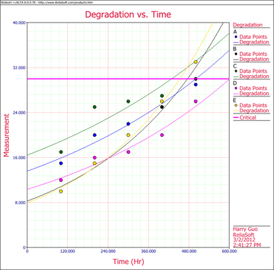
These results are shown graphically in the next figure.
[math]\displaystyle{ }[/math]
These values can now be substituted into the underlying exponential model, solved for [math]\displaystyle{ x }[/math] or:
Using the values of [math]\displaystyle{ a }[/math] and [math]\displaystyle{ b }[/math] , with [math]\displaystyle{ y=30 }[/math] , the resulting time at which the crack length reaches 30mm is then found for each sample:
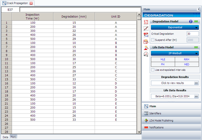
These cycles-to-failure can now be analyzed in the conventional manner. Assuming a two-parameter Weibull distribution and using the MLE estimation method, the distribution parameters are calculated as [math]\displaystyle{ \beta =8.055 }[/math] and [math]\displaystyle{ \eta =519,555. }[/math] Using these values, the B10 life is calculated to be 392,918 cycles. The degradation analysis tool in Weibull++ performs this type of analysis for you. The following figure shows the data as entered in Weibull++ for this analysis.
[math]\displaystyle{ }[/math]


