Arrhenius Relationship: Difference between revisions
| Line 87: | Line 87: | ||
{{alta al}} | {{alta al}} | ||
{{arrhenius confidence bounds}} | |||
Revision as of 22:14, 12 January 2012
Introduction
The Arrhenius life-stress model (or relationship) is probably the most common life-stress relationship utilized in accelerated life testing. It has been widely used when the stimulus or acceleration variable (or stress) is thermal (i.e. temperature). It is derived from the Arrhenius reaction rate equation proposed by the Swedish physical chemist Svandte Arrhenius in 1887.
Introduction
The Arrhenius life-stress model (or relationship) is probably the most common life-stress relationship utilized in accelerated life testing. It has been widely used when the stimulus or acceleration variable (or stress) is thermal (i.e. temperature). It is derived from the Arrhenius reaction rate equation proposed by the Swedish physical chemist Svandte Arrhenius in 1887. Template loop detected: Template:Arrhenius formulation
Life Stress Plots
The Arrhenius relationship can be linearized and plotted on a Life vs. Stress plot, also called the Arrhenius plot. The relationship is linearized by taking the natural logarithm of both sides in Eqn. (arrhenius) or:
- [math]\displaystyle{ ln(L(V))=ln(C)+\frac{B}{V} }[/math]
- [math]\displaystyle{ }[/math]
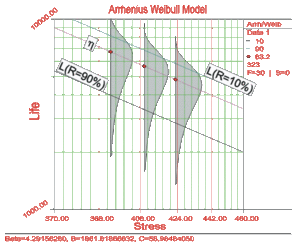
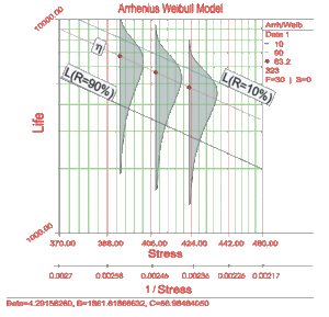
In Eqn. (log-arrh) [math]\displaystyle{ \ln (C) }[/math] is the intercept of the line and [math]\displaystyle{ B }[/math] is the slope of the line. Note that the inverse of the stress, and not the stress, is the variable. In Fig. 2, life is plotted versus stress and not versus the inverse stress. This is because Eqn. (log-arrh) was plotted on a reciprocal scale. On such a scale, the slope [math]\displaystyle{ B }[/math] appears to be negative even though it has a positive value. This is because [math]\displaystyle{ B }[/math] is actually the slope of the reciprocal of the stress and not the slope of the stress. The reciprocal of the stress is decreasing as stress is increasing ( [math]\displaystyle{ \tfrac{1}{V} }[/math] is decreasing as [math]\displaystyle{ V }[/math] is increasing). The two different axes are shown in Fig. 3.
- [math]\displaystyle{ }[/math]
The Arrhenius relationship is plotted on a reciprocal scale for practical reasons. For example, in Fig. 3 it is more convenient to locate the life corresponding to a stress level of 370K than to take the reciprocal of 370K (0.0027) first, and then locate the corresponding life.
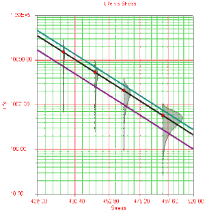
The shaded areas shown in Fig. 3 are the imposed at each test stress level. From such imposed [math]\displaystyle{ pdfs }[/math] one can see the range of the life at each test stress level, as well as the scatter in life. The next figure (Fig. 4) illustrates a case in which there is a significant scatter in life at each of the test stress levels.
- [math]\displaystyle{ }[/math]
Activation Energy and the Parameter B
Depending on the application (and where the stress is exclusively thermal), the parameter [math]\displaystyle{ B }[/math] can be replaced by:
- [math]\displaystyle{ B=\frac{{{E}_{A}}}{K}=\frac{\text{activation energy}}{\text{Boltzma}{{\text{n}}^{\prime }}\text{s constant}}=\frac{\text{activation energy}}{8.623\times {{10}^{-5}}\text{eV}{{\text{K}}^{-1}}} }[/math]
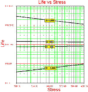
Note that in this formulation, the activation energy [math]\displaystyle{ {{E}_{A}} }[/math] must be known a priori. If the activation energy is known then there is only one model parameter remaining, [math]\displaystyle{ C. }[/math] Because in most real life situations this is rarely the case, all subsequent formulations will assume that this activation energy is unknown and treat [math]\displaystyle{ B }[/math] as one of the model parameters. As it can be seen in Eqn. (arrhenius), [math]\displaystyle{ B }[/math] has the same properties as the activation energy. In other words, [math]\displaystyle{ B }[/math] is a measure of the effect that the stress (i.e. temperature) has on the life. The larger the value of [math]\displaystyle{ B, }[/math] the higher the dependency of the life on the specific stress (see Fig. 5). Parameter [math]\displaystyle{ B }[/math] may also take negative values. In that case, life is increasing with increasing stress (see Fig. 5). An example of this would be plasma filled bulbs, where low temperature is a higher stress on the bulbs than high temperature.
- [math]\displaystyle{ }[/math]
Template loop detected: Template:A-a acceleration
Template loop detected: Template:Aae
Template loop detected: Template:Aaw
Example
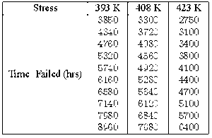
Consider the following times-to-failure data at three different stress levels.
The data set was analyzed jointly and with a complete MLE solution over the entire data set, using ReliaSoft's ALTA. The analysis yields:
- [math]\displaystyle{ \widehat{\beta }=4.2915822 }[/math]
- [math]\displaystyle{ \widehat{B}=1861.6186657 }[/math]
- [math]\displaystyle{ \widehat{C}=58.9848692 }[/math]
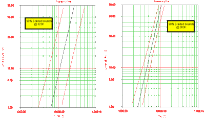
Once the parameters of the model are estimated, extrapolation and other life measures can be directly obtained using the appropriate equations. Using the MLE method, confidence bounds for all estimates can be obtained. Note in Fig. 10 that the more distant the accelerated stress from the operating stress, the greater the uncertainty of the extrapolation. The degree of uncertainty is reflected in the confidence bounds. (General theory and calculations for confidence intervals are presented in Appendix A. Specific calculations for confidence bounds on the Arrhenius model are presented in Appendix 6.A following this chapter.)
Template loop detected: Template:Alta al
Template loop detected: Template:Arrhenius confidence bounds
Life Stress Plots
The Arrhenius relationship can be linearized and plotted on a Life vs. Stress plot, also called the Arrhenius plot. The relationship is linearized by taking the natural logarithm of both sides in Eqn. (arrhenius) or:
- [math]\displaystyle{ ln(L(V))=ln(C)+\frac{B}{V} }[/math]
- [math]\displaystyle{ }[/math]
In Eqn. (log-arrh) [math]\displaystyle{ \ln (C) }[/math] is the intercept of the line and [math]\displaystyle{ B }[/math] is the slope of the line. Note that the inverse of the stress, and not the stress, is the variable. In Fig. 2, life is plotted versus stress and not versus the inverse stress. This is because Eqn. (log-arrh) was plotted on a reciprocal scale. On such a scale, the slope [math]\displaystyle{ B }[/math] appears to be negative even though it has a positive value. This is because [math]\displaystyle{ B }[/math] is actually the slope of the reciprocal of the stress and not the slope of the stress. The reciprocal of the stress is decreasing as stress is increasing ( [math]\displaystyle{ \tfrac{1}{V} }[/math] is decreasing as [math]\displaystyle{ V }[/math] is increasing). The two different axes are shown in Fig. 3.
- [math]\displaystyle{ }[/math]
The Arrhenius relationship is plotted on a reciprocal scale for practical reasons. For example, in Fig. 3 it is more convenient to locate the life corresponding to a stress level of 370K than to take the reciprocal of 370K (0.0027) first, and then locate the corresponding life.
The shaded areas shown in Fig. 3 are the imposed at each test stress level. From such imposed [math]\displaystyle{ pdfs }[/math] one can see the range of the life at each test stress level, as well as the scatter in life. The next figure (Fig. 4) illustrates a case in which there is a significant scatter in life at each of the test stress levels.
- [math]\displaystyle{ }[/math]
Activation Energy and the Parameter B
Depending on the application (and where the stress is exclusively thermal), the parameter [math]\displaystyle{ B }[/math] can be replaced by:
- [math]\displaystyle{ B=\frac{{{E}_{A}}}{K}=\frac{\text{activation energy}}{\text{Boltzma}{{\text{n}}^{\prime }}\text{s constant}}=\frac{\text{activation energy}}{8.623\times {{10}^{-5}}\text{eV}{{\text{K}}^{-1}}} }[/math]
Note that in this formulation, the activation energy [math]\displaystyle{ {{E}_{A}} }[/math] must be known a priori. If the activation energy is known then there is only one model parameter remaining, [math]\displaystyle{ C. }[/math] Because in most real life situations this is rarely the case, all subsequent formulations will assume that this activation energy is unknown and treat [math]\displaystyle{ B }[/math] as one of the model parameters. As it can be seen in Eqn. (arrhenius), [math]\displaystyle{ B }[/math] has the same properties as the activation energy. In other words, [math]\displaystyle{ B }[/math] is a measure of the effect that the stress (i.e. temperature) has on the life. The larger the value of [math]\displaystyle{ B, }[/math] the higher the dependency of the life on the specific stress (see Fig. 5). Parameter [math]\displaystyle{ B }[/math] may also take negative values. In that case, life is increasing with increasing stress (see Fig. 5). An example of this would be plasma filled bulbs, where low temperature is a higher stress on the bulbs than high temperature.
- [math]\displaystyle{ }[/math]
Introduction
The Arrhenius life-stress model (or relationship) is probably the most common life-stress relationship utilized in accelerated life testing. It has been widely used when the stimulus or acceleration variable (or stress) is thermal (i.e. temperature). It is derived from the Arrhenius reaction rate equation proposed by the Swedish physical chemist Svandte Arrhenius in 1887. Template loop detected: Template:Arrhenius formulation
Life Stress Plots
The Arrhenius relationship can be linearized and plotted on a Life vs. Stress plot, also called the Arrhenius plot. The relationship is linearized by taking the natural logarithm of both sides in Eqn. (arrhenius) or:
- [math]\displaystyle{ ln(L(V))=ln(C)+\frac{B}{V} }[/math]
- [math]\displaystyle{ }[/math]
In Eqn. (log-arrh) [math]\displaystyle{ \ln (C) }[/math] is the intercept of the line and [math]\displaystyle{ B }[/math] is the slope of the line. Note that the inverse of the stress, and not the stress, is the variable. In Fig. 2, life is plotted versus stress and not versus the inverse stress. This is because Eqn. (log-arrh) was plotted on a reciprocal scale. On such a scale, the slope [math]\displaystyle{ B }[/math] appears to be negative even though it has a positive value. This is because [math]\displaystyle{ B }[/math] is actually the slope of the reciprocal of the stress and not the slope of the stress. The reciprocal of the stress is decreasing as stress is increasing ( [math]\displaystyle{ \tfrac{1}{V} }[/math] is decreasing as [math]\displaystyle{ V }[/math] is increasing). The two different axes are shown in Fig. 3.
- [math]\displaystyle{ }[/math]
The Arrhenius relationship is plotted on a reciprocal scale for practical reasons. For example, in Fig. 3 it is more convenient to locate the life corresponding to a stress level of 370K than to take the reciprocal of 370K (0.0027) first, and then locate the corresponding life.
The shaded areas shown in Fig. 3 are the imposed at each test stress level. From such imposed [math]\displaystyle{ pdfs }[/math] one can see the range of the life at each test stress level, as well as the scatter in life. The next figure (Fig. 4) illustrates a case in which there is a significant scatter in life at each of the test stress levels.
- [math]\displaystyle{ }[/math]
Activation Energy and the Parameter B
Depending on the application (and where the stress is exclusively thermal), the parameter [math]\displaystyle{ B }[/math] can be replaced by:
- [math]\displaystyle{ B=\frac{{{E}_{A}}}{K}=\frac{\text{activation energy}}{\text{Boltzma}{{\text{n}}^{\prime }}\text{s constant}}=\frac{\text{activation energy}}{8.623\times {{10}^{-5}}\text{eV}{{\text{K}}^{-1}}} }[/math]
Note that in this formulation, the activation energy [math]\displaystyle{ {{E}_{A}} }[/math] must be known a priori. If the activation energy is known then there is only one model parameter remaining, [math]\displaystyle{ C. }[/math] Because in most real life situations this is rarely the case, all subsequent formulations will assume that this activation energy is unknown and treat [math]\displaystyle{ B }[/math] as one of the model parameters. As it can be seen in Eqn. (arrhenius), [math]\displaystyle{ B }[/math] has the same properties as the activation energy. In other words, [math]\displaystyle{ B }[/math] is a measure of the effect that the stress (i.e. temperature) has on the life. The larger the value of [math]\displaystyle{ B, }[/math] the higher the dependency of the life on the specific stress (see Fig. 5). Parameter [math]\displaystyle{ B }[/math] may also take negative values. In that case, life is increasing with increasing stress (see Fig. 5). An example of this would be plasma filled bulbs, where low temperature is a higher stress on the bulbs than high temperature.
- [math]\displaystyle{ }[/math]
Template loop detected: Template:A-a acceleration
Template loop detected: Template:Aae
Template loop detected: Template:Aaw
Example
Consider the following times-to-failure data at three different stress levels.
The data set was analyzed jointly and with a complete MLE solution over the entire data set, using ReliaSoft's ALTA. The analysis yields:
- [math]\displaystyle{ \widehat{\beta }=4.2915822 }[/math]
- [math]\displaystyle{ \widehat{B}=1861.6186657 }[/math]
- [math]\displaystyle{ \widehat{C}=58.9848692 }[/math]
Once the parameters of the model are estimated, extrapolation and other life measures can be directly obtained using the appropriate equations. Using the MLE method, confidence bounds for all estimates can be obtained. Note in Fig. 10 that the more distant the accelerated stress from the operating stress, the greater the uncertainty of the extrapolation. The degree of uncertainty is reflected in the confidence bounds. (General theory and calculations for confidence intervals are presented in Appendix A. Specific calculations for confidence bounds on the Arrhenius model are presented in Appendix 6.A following this chapter.)
Template loop detected: Template:Alta al
Template loop detected: Template:Arrhenius confidence bounds
Example
Consider the following times-to-failure data at three different stress levels.
The data set was analyzed jointly and with a complete MLE solution over the entire data set, using ReliaSoft's ALTA. The analysis yields:
- [math]\displaystyle{ \widehat{\beta }=4.2915822 }[/math]
- [math]\displaystyle{ \widehat{B}=1861.6186657 }[/math]
- [math]\displaystyle{ \widehat{C}=58.9848692 }[/math]
Once the parameters of the model are estimated, extrapolation and other life measures can be directly obtained using the appropriate equations. Using the MLE method, confidence bounds for all estimates can be obtained. Note in Fig. 10 that the more distant the accelerated stress from the operating stress, the greater the uncertainty of the extrapolation. The degree of uncertainty is reflected in the confidence bounds. (General theory and calculations for confidence intervals are presented in Appendix A. Specific calculations for confidence bounds on the Arrhenius model are presented in Appendix 6.A following this chapter.)
Introduction
The Arrhenius life-stress model (or relationship) is probably the most common life-stress relationship utilized in accelerated life testing. It has been widely used when the stimulus or acceleration variable (or stress) is thermal (i.e. temperature). It is derived from the Arrhenius reaction rate equation proposed by the Swedish physical chemist Svandte Arrhenius in 1887. Template loop detected: Template:Arrhenius formulation
Life Stress Plots
The Arrhenius relationship can be linearized and plotted on a Life vs. Stress plot, also called the Arrhenius plot. The relationship is linearized by taking the natural logarithm of both sides in Eqn. (arrhenius) or:
- [math]\displaystyle{ ln(L(V))=ln(C)+\frac{B}{V} }[/math]
- [math]\displaystyle{ }[/math]
In Eqn. (log-arrh) [math]\displaystyle{ \ln (C) }[/math] is the intercept of the line and [math]\displaystyle{ B }[/math] is the slope of the line. Note that the inverse of the stress, and not the stress, is the variable. In Fig. 2, life is plotted versus stress and not versus the inverse stress. This is because Eqn. (log-arrh) was plotted on a reciprocal scale. On such a scale, the slope [math]\displaystyle{ B }[/math] appears to be negative even though it has a positive value. This is because [math]\displaystyle{ B }[/math] is actually the slope of the reciprocal of the stress and not the slope of the stress. The reciprocal of the stress is decreasing as stress is increasing ( [math]\displaystyle{ \tfrac{1}{V} }[/math] is decreasing as [math]\displaystyle{ V }[/math] is increasing). The two different axes are shown in Fig. 3.
- [math]\displaystyle{ }[/math]
The Arrhenius relationship is plotted on a reciprocal scale for practical reasons. For example, in Fig. 3 it is more convenient to locate the life corresponding to a stress level of 370K than to take the reciprocal of 370K (0.0027) first, and then locate the corresponding life.
The shaded areas shown in Fig. 3 are the imposed at each test stress level. From such imposed [math]\displaystyle{ pdfs }[/math] one can see the range of the life at each test stress level, as well as the scatter in life. The next figure (Fig. 4) illustrates a case in which there is a significant scatter in life at each of the test stress levels.
- [math]\displaystyle{ }[/math]
Activation Energy and the Parameter B
Depending on the application (and where the stress is exclusively thermal), the parameter [math]\displaystyle{ B }[/math] can be replaced by:
- [math]\displaystyle{ B=\frac{{{E}_{A}}}{K}=\frac{\text{activation energy}}{\text{Boltzma}{{\text{n}}^{\prime }}\text{s constant}}=\frac{\text{activation energy}}{8.623\times {{10}^{-5}}\text{eV}{{\text{K}}^{-1}}} }[/math]
Note that in this formulation, the activation energy [math]\displaystyle{ {{E}_{A}} }[/math] must be known a priori. If the activation energy is known then there is only one model parameter remaining, [math]\displaystyle{ C. }[/math] Because in most real life situations this is rarely the case, all subsequent formulations will assume that this activation energy is unknown and treat [math]\displaystyle{ B }[/math] as one of the model parameters. As it can be seen in Eqn. (arrhenius), [math]\displaystyle{ B }[/math] has the same properties as the activation energy. In other words, [math]\displaystyle{ B }[/math] is a measure of the effect that the stress (i.e. temperature) has on the life. The larger the value of [math]\displaystyle{ B, }[/math] the higher the dependency of the life on the specific stress (see Fig. 5). Parameter [math]\displaystyle{ B }[/math] may also take negative values. In that case, life is increasing with increasing stress (see Fig. 5). An example of this would be plasma filled bulbs, where low temperature is a higher stress on the bulbs than high temperature.
- [math]\displaystyle{ }[/math]
Template loop detected: Template:A-a acceleration
Template loop detected: Template:Aae
Template loop detected: Template:Aaw
Example
Consider the following times-to-failure data at three different stress levels.
The data set was analyzed jointly and with a complete MLE solution over the entire data set, using ReliaSoft's ALTA. The analysis yields:
- [math]\displaystyle{ \widehat{\beta }=4.2915822 }[/math]
- [math]\displaystyle{ \widehat{B}=1861.6186657 }[/math]
- [math]\displaystyle{ \widehat{C}=58.9848692 }[/math]
Once the parameters of the model are estimated, extrapolation and other life measures can be directly obtained using the appropriate equations. Using the MLE method, confidence bounds for all estimates can be obtained. Note in Fig. 10 that the more distant the accelerated stress from the operating stress, the greater the uncertainty of the extrapolation. The degree of uncertainty is reflected in the confidence bounds. (General theory and calculations for confidence intervals are presented in Appendix A. Specific calculations for confidence bounds on the Arrhenius model are presented in Appendix 6.A following this chapter.)
Template loop detected: Template:Alta al
Template loop detected: Template:Arrhenius confidence bounds

