Additional Tools

Additional Tools

ALTA and ALTA PRO contain some additional analysis tools that allow you to perform supplementary analyses. These include tests of comparison between two data sets, likelihood ratio tests, degradation analysis and accelerated test planning. The principles and theory behind each of these analysis tools are presented next.

Common Shape Parameter Likelihood Ratio Test

In order to assess the assumption of a common shape parameter among the data obtained at various stress levels, the likelihood ratio (LR) test can be utilized [28]. This test applies to any distribution with a shape parameter. In the case of ALTA, it applies to the Weibull and lognormal distributions. When Weibull is used as the underlying life distribution, the shape parameter, [math]\displaystyle{ \beta , }[/math] is assumed to be constant across the different stress levels (i.e. stress independent). Similarly[math]\displaystyle{ {{\sigma }_{{{T}'}}} }[/math], the parameter of the lognormal distribution is assumed to be constant across the different stress levels. The likelihood ratio test is performed by first obtaining the LR test statistic, [math]\displaystyle{ T }[/math] . If the true shape parameters are equal, then the distribution of [math]\displaystyle{ T }[/math] is approximately chi-square with [math]\displaystyle{ n-1 }[/math] degrees of freedom, where [math]\displaystyle{ n }[/math] is the number of test stress levels with two or more exact failure points. The LR test statistic, [math]\displaystyle{ T }[/math] , is calculated as follows:

[math]\displaystyle{ T=2({{\hat{\Lambda }}_{1}}+...+{{\hat{\Lambda }}_{n}}-{{\hat{\Lambda }}_{0}}) }[/math]

are the likelihood values obtained by fitting a separate distribution to the data from each of the [math]\displaystyle{ n }[/math] test stress levels (with two or more exact failure times). The likelihood value, [math]\displaystyle{ {{\hat{\Lambda }}_{0}}, }[/math] is obtained by fitting a model with a common shape parameter and a separate scale parameter for each of the [math]\displaystyle{ n }[/math] stress levels, using indicator variables.
Once the LR statistic has been calculated, then:

• If [math]\displaystyle{ T\le {{\chi }^{2}}(1-\alpha ;n-1), }[/math] the [math]\displaystyle{ n }[/math] shape parameter estimates do not differ statistically significantly at the 100 [math]\displaystyle{ \alpha % }[/math] level. • If [math]\displaystyle{ T\gt {{\chi }^{2}}(1-\alpha ;n-1), }[/math] the [math]\displaystyle{ n }[/math] shape parameter estimates differ statistically significantly at the 100 [math]\displaystyle{ \alpha % }[/math] level. [math]\displaystyle{ {{\chi }^{2}}(1-\alpha ;n-1) }[/math] is the 100(1- [math]\displaystyle{ \alpha ) }[/math] percentile of the chi-square distribution with [math]\displaystyle{ n-1 }[/math] degrees of freedom.

Example

Consider the following times-to-failure data at three different stress levels.

Stress	406 K	416 K	426 K
Time Failed (hrs)	248	164	92
	456	176	105
	528	289	155
	731	319	184
	813	340	219
		543	235

The data set was analyzed using an Arrhenius-Weibull model. The analysis yields:

[math]\displaystyle{ \widehat{\beta }=2.9658 }[/math]

[math]\displaystyle{ \widehat{C}=2.3966\cdot {{10}^{-9}} }[/math]

The assumption of a common [math]\displaystyle{ \beta }[/math] across the different stress levels can be assessed visually using a probability plot.

Probability plot of the threee test stress levels.

In Fig. 1, it can be seen that the plotted data from the different stress levels seem to be fairly parallel.

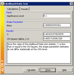
A better assessment can be made with the LR test, which can be performed using the Likelihood Ratio Test tool in ALTA. For example, in the following figure, the [math]\displaystyle{ \beta s }[/math] are compared for equality at the 10% level.

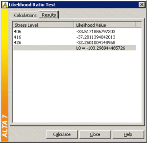
The individual likelihood values for each of the test stresses can be found in the Results tab of the Likelihood Ratio Test window.

The LR test statistic, [math]\displaystyle{ T }[/math] , is calculated to be 0.481. Therefore, [math]\displaystyle{ T=0.481\le 4.605={{\chi }^{2}}(0.9;2), }[/math] the [math]\displaystyle{ {\beta }' }[/math] s do not differ significantly at the [math]\displaystyle{ 10% }[/math] level.

Tests of Comparison

It is often desirable to be able to compare two sets of accelerated life data in order to determine which of the data sets has a more favorable life distribution. The units from which the data are obtained could either be from two alternate designs, alternate manufacturers or alternate lots or assembly lines. Many methods are available in statistical literature for doing this when the units come from a complete sample, i.e. a sample with no censoring. This process becomes a little more difficult when dealing with data sets that have censoring, or when trying to compare two data sets that have different distributions. In general, the problem boils down to that of being able to determine any statistically significant difference between the two samples of potentially censored data from two possibly different populations. This section discusses some of the methods that are applicable to censored data, and are available in ALTA.

Simple Plotting

One popular graphical method for making this determination involves plotting the data at a given stress level with confidence bounds and seeing whether the bounds overlap or separate at the point of interest. This can be effective for comparisons at a given point in time or a given reliability level, but it is difficult to assess the overall behavior of the two distributions, as the confidence bounds may overlap at some points and be far apart at others. This can be easily done using the multiple plot feature in ALTA.

Estimating [math]\displaystyle{ P\left[ {{t}_{2}}\ge {{t}_{1}} \right] }[/math] Using the Comparison Wizard

Another methodology, suggested by Gerald G. Brown and Herbert C. Rutemiller, is to estimate the probability of whether the times-to-failure of one population are better or worse than the times-to-failure of the second. The equation used to estimate this probability is given by:

[math]\displaystyle{ P\left[ {{t}_{2}}\ge {{t}_{1}} \right]=\mathop{}_{0}^{\infty }{{f}_{1}}(t)\cdot {{R}_{2}}(t)\cdot dt }[/math]

where [math]\displaystyle{ {{f}_{1}}(t) }[/math] is the [math]\displaystyle{ pdf }[/math] of the first distribution and [math]\displaystyle{ {{R}_{2}}(t) }[/math] is the reliability function of the second distribution. The evaluation of the superior data set is based on whether this probability is smaller or greater than 0.50. If the probability is equal to 0.50, that is equivalent to saying that the two distributions are identical.
If given two alternate designs with life test data, where X and Y represent the life test data from two different populations, and if we simply wanted to choose the component at time [math]\displaystyle{ t }[/math] with the higher reliability, one choice would be to select the component with the higher reliability at time [math]\displaystyle{ t }[/math] . However, if we wanted to design a product as long-lived as possible, we would want to calculate the probability that the entire distribution of one product is better than the other and choose X or Y when this probability is above or below 0.50 respectively.
The statement ``the probability that X is greater than or equal to Y can be interpreted as follows:
• If [math]\displaystyle{ P=0.50 }[/math] , then the statement is equivalent to saying that both X and Y are equal.
• If [math]\displaystyle{ P\lt 0.50 }[/math] or, for example, [math]\displaystyle{ P=0.10 }[/math] , then the statement is equivalent to saying that [math]\displaystyle{ P=1-0.10=0.90 }[/math] , or Y is better than X with a 90% probability.
ALTA's Comparison Wizard allows you to perform such calculations. The comparison is performed at the given use stress levels of each data set. Eqn. (eqnStress) can then be expressed as:

[math]\displaystyle{ P\left[ {{t}_{2}}\ge {{t}_{1}} \right]=\mathop{}_{0}^{\infty }{{f}_{1}}(t,{{V}_{Use,1}})\cdot {{R}_{2}}(t,{{V}_{Use,2}})\cdot dt }[/math]

The disadvantage of this method is that the sample sizes are not taken into account, thus one should avoid using this method of comparison when the sample sizes are different.

Degradation Analysis

Given that products are frequently being designed with higher reliabilities and developed in shorter amounts of time, even accelerated life testing is often not sufficient to yield reliability results in the desired timeframe. In some cases, it is possible to infer the reliability behavior of unfailed test samples with only the accumulated test time information and assumptions about the distribution. However, this generally leads to a great deal of uncertainty in the results. Another option in this situation is the use of degradation analysis. Degradation analysis involves the measurement and extrapolation of degradation or performance data that can be directly related to the presumed failure of the product in question. Many failure mechanisms can be directly linked to the degradation of part of the product, and degradation analysis allows the user to extrapolate to an assumed failure time based on the measurements of degradation or performance over time. To reduce testing time even further, tests can be performed at elevated stresses and the degradation at these elevated stresses can be measured resulting in a type of analysis known as accelerated degradation. In some cases, it is possible to directly measure the degradation over time, as with the wear of brake pads or with the propagation of crack size. In other cases, direct measurement of degradation might not be possible without invasive or destructive measurement techniques that would directly affect the subsequent performance of the product. In such cases, the degradation of the product can be estimated through the measurement of certain performance characteristics, such as using resistance to gauge the degradation of a dielectric material. In either case, however, it is necessary to be able to define a level of degradation or performance at which a failure is said to have occurred. With this failure level of performance defined, it is a relatively simple matter to use basic mathematical models to extrapolate the performance measurements over time to the point where the failure is said to occur. This is done at different stress levels, and therefore each time-to-failure is also associated with a corresponding stress level. Once the times-to-failure at the corresponding stress levels have been determined, it is merely a matter of analyzing the extrapolated failure times in the same manner as you would conventional accelerated time-to-failure data.
Once the level of failure (or the degradation level that would constitute a failure) is defined, the degradation for multiple units over time needs to be measured (with different groups of units being at different stress levels). As with conventional accelerated data, the amount of certainty in the results is directly related to the number of units being tested, the number of units at each stress level, as well as in the amount of overstressing with respect to the normal operating conditions. The performance or degradation of these units needs to be measured over time, either continuously or at predetermined intervals. Once this information has been recorded, the next task is to extrapolate the performance measurements to the defined failure level in order to estimate the failure time. ALTA allows the user to perform such analysis using a linear, exponential, power, logarithmic, Gompertz or Lloyd-Lipow model to perform this extrapolation. These models have the following forms:

[math]\displaystyle{ \begin{matrix} Linear\ \ : & y=a\cdot x+b \\ Exponential\ \ : & y=b\cdot {{e}^{a\cdot x}} \\ Power\ \ : & y=b\cdot {{x}^{a}} \\ Logarithmic\ \ : & y=a\cdot ln(x)+b \\ Gompertz\ \ : & y=a\cdot {{b}^{cx}} \\ Lloyd-Lipow\ \ : & y=a-b/x \\ \end{matrix} }[/math]

where [math]\displaystyle{ y }[/math] represents the performance, [math]\displaystyle{ x }[/math] represents time, and [math]\displaystyle{ a }[/math] and [math]\displaystyle{ b }[/math] are model parameters to be solved for. Once the model parameters [math]\displaystyle{ {{a}_{i}} }[/math] and [math]\displaystyle{ {{b}_{i}} }[/math] (and [math]\displaystyle{ {{c}_{i}} }[/math] for Lloyd-Lipow) are estimated for each sample [math]\displaystyle{ i }[/math] , a time, [math]\displaystyle{ {{x}_{i}}, }[/math] can be extrapolated that corresponds to the defined level of failure [math]\displaystyle{ y }[/math] . The computed [math]\displaystyle{ {{x}_{i}} }[/math] can now be used as our times-to-failure for subsequent accelerated life data analysis. As with any sort of extrapolation, one must be careful not to extrapolate too far beyond the actual range of data in order to avoid large inaccuracies (modeling errors).

One may also define a censoring time past which no failure times are extrapolated. In practice, there is usually a rather narrow band in which this censoring time has any practical meaning. With a relatively low censoring time, no failure times will be extrapolated, which defeats the purpose of degradation analysis. A relatively high censoring time would occur after all of the theoretical failure times, thus being rendered meaningless. Nevertheless, certain situations may arise in which it is beneficial to be able to censor the accelerated degradation data.

Example

Consider a chemical solution (e.g. ink formulation, medicine, etc.) that degrades with time. A quantitative measure of the quality of the product can be obtained. This measure (QM) is said to be around 100 when the product is first manufactured and decreases with product age. The minimum acceptable value for QM is 50. Products with QM equal to or lower than 50 are considered to be out of compliance or failed.
Engineering analysis has indicated that at higher temperatures the QM has a higher rate of decrease. Assuming that the product's normal use temperature is 20º C (or 293K), the goal is to determine the shelf life of the product via an accelerated degradation test. For the purpose of this analysis ``shelf life is defined as the time by which 10% of the products will have a QM that is out of compliance. 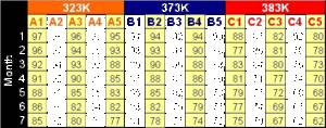For this experiment, 15 samples of the product were tested, with 5 samples in each of three accelerated stress environments: 323K, 373K and 383K. Once a month, and for a period of seven months, the QM for each sample was measured and recorded. The data obtained is given in Table 1.

Table 1: Accelerated Degradation Data

Since all of the readings are above the critical QM threshold of 50, none of the samples tested in this experiment had gone out of compliance (or failed) by the end of the test. However, there was sufficient data for the degradation of each sample to extrapolate a time-to-failure (i.e. the month at which we expect each sample to be at QM=50).

Data entered in ALTA's Degradation Analysis Folio.

Using ALTA's Degradation Analysis Folio (shown in Fig. 2) the data for all samples were entered and individually fitted to multiple exponential curves. Fig. 3 shows sample graphs. From each respective curve, a time-to-failure (i.e. the time the product is expected to go out of compliance) was automatically extrapolated and transferred to an ALTA Standard Folio (Fig. 4).

Sample degradation lines.

Extrapolated time-to-failure data in the ALTA PRO Standard Folio.

Several plots can be obtained from the analysis. Specifically, Fig. 5 shows a Weibull probability plot at the use stress level. Fig. 6 shows a Life vs. Stress plot where the line represents the time by which 10% of the units are expected to be out of compliance (at a given temperature).

Use Level Weibull probability plot.

Life vs. Stress plot.

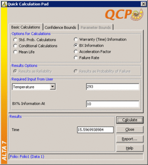
Based on this analysis, the projected shelf life of this product is 15.6 months. The desired result could also have been obtained from the QCP, as shown next.

Accelerated Life Test Plans

Poor accelerated test plans waste time, effort and money and may not even yield the desired information. Before starting an accelerated test (which is sometimes an expensive and difficult endeavor), it is advisable to have a plan that helps in acurately estimating reliability at operating conditions while minimizing test time and costs. A test plan should be used to decide on the appropriate stress levels that should be used (for each stress type) and the amount of the test units that need to be allocated to the different stress levels (for each combination of the different stress types' levels). This section presents some common test plans for one-stress and two-stress accelerated tests.

General Assumptions

Most accelerated life testing plans use the following model and testing assumptions that correspond to many practical quantitative accelerated life testing problems. 1. The log-time-to-failure for each unit follows a location-scale distribution such that:

[math]\displaystyle{ \underset{}{\overset{}{\mathop{\Pr }}}\,(Y\le y)=\Phi \left( \frac{y-\mu }{\sigma } \right) }[/math]

where [math]\displaystyle{ \mu }[/math] and [math]\displaystyle{ \sigma }[/math] are the location and scale parameters respectively and [math]\displaystyle{ \Phi }[/math] ( [math]\displaystyle{ \cdot }[/math] ) is the standard form of the location-scale distribution.
2. Failure times for all test units, at all stress levels, are statistically independent.
3. The location parameter [math]\displaystyle{ \mu }[/math] is a linear function of stress. Specifically, it is assumed that:

[math]\displaystyle{ \mu =\mu ({{z}_{1}})={{\gamma }_{0}}+{{\gamma }_{1}}x }[/math]

4. The scale parameter, [math]\displaystyle{ \sigma , }[/math] does not depend on the stress levels. All units are tested until a pre-specified test time.
5. Two of the most common models used in quantitative accelerated life testing are the linear Weibull and lognormal models. The Weibull model is given by:

[math]\displaystyle{ Y\sim SEV\left[ \mu (z)={{\gamma }_{0}}+{{\gamma }_{1}}x,\sigma \right] }[/math]

where [math]\displaystyle{ SEV }[/math] denotes the smallest extreme value distribution. The lognormal model is given by:

[math]\displaystyle{ Y\sim Normal\left[ \mu (z)={{\gamma }_{0}}+{{\gamma }_{1}}z,\sigma \right] }[/math]

That is, log life [math]\displaystyle{ Y }[/math] is assumed to have either an [math]\displaystyle{ SEV }[/math] or a normal distribution with location parameter [math]\displaystyle{ \mu (z) }[/math] , expressed as a linear function of [math]\displaystyle{ z }[/math] and constant scale parameter [math]\displaystyle{ \sigma }[/math] .

Planning Criteria and Problem Formulation

Without loss of generality, a stress can be standardized as follows:

[math]\displaystyle{ \xi =\frac{x-{{x}_{D}}}{{{x}_{H}}-{{x}_{D}}} }[/math]

where:
• [math]\displaystyle{ {{x}_{D}} }[/math] is the use stress or design stress at which product life is of primary interest. • [math]\displaystyle{ {{x}_{H}} }[/math] is the highest test stress level. The values of [math]\displaystyle{ x }[/math] , [math]\displaystyle{ {{x}_{D}} }[/math] and [math]\displaystyle{ {{x}_{H}} }[/math] refer to the actual values of stress or to the transformed values in case a transformation (e.g. the reciprocal transformation to obtain the Arrhenius relationship or the log transformation to obtain the power relationship) is used.

Typically, there will be a limit on the highest level of stress for testing because the distribution and life-stress relationship assumptions hold only for a limited range of the stress. The highest test level of stress, [math]\displaystyle{ {{x}_{H}}, }[/math] can be determined based on engineering knowledge, preliminary tests or experience with similar products. Higher stresses will help end the test faster, but might violate your distribution and life-stress relationship assumptions.
Therefore, [math]\displaystyle{ \xi =0 }[/math] at the design stress and [math]\displaystyle{ \xi =1 }[/math] at the highest test stress.
A common purpose of an accelerated life test experiment is to estimate a particular percentile (unreliability value of [math]\displaystyle{ p }[/math] ), [math]\displaystyle{ {{T}_{p}} }[/math] , in the lower tail of the failure distribution at use stress. Thus a natural criterion is to minimize [math]\displaystyle{ Var({{\hat{T}}_{p}}) }[/math] or [math]\displaystyle{ Var({{\hat{Y}}_{p}}) }[/math] such that [math]\displaystyle{ {{Y}_{p}}=\ln ({{T}_{p}}) }[/math] . [math]\displaystyle{ Var({{\hat{Y}}_{p}}) }[/math] measures the precision of the [math]\displaystyle{ p }[/math] quantile estimator; smaller values mean less variation in the value of [math]\displaystyle{ {{\hat{Y}}_{p}} }[/math] in repeated samplings. Hence a good test plan should yield a relatively small, if not the minimum, [math]\displaystyle{ Var({{\hat{Y}}_{p}}) }[/math] value. For the minimization problem, the decision variables are [math]\displaystyle{ {{\xi }_{i}} }[/math] (the standardized stress level used in the test) and [math]\displaystyle{ {{\pi }_{i}} }[/math] (the percentage of the total test units allocated at that level). The optimization problem can be formulized as follows.
Minimize:

[math]\displaystyle{ Var({{\hat{Y}}_{p}})=f({{\xi }_{i}},{{\pi }_{i}}) }[/math]

Subject to:

[math]\displaystyle{ 0\le {{\pi }_{i}}\le 1,\text{ }i=1,2,...n }[/math]

where:

[math]\displaystyle{ \underset{i=1}{\overset{n}{\mathop{\sum }}}\,{{\pi }_{i}}=1 }[/math]

vAn optimum accelerated test plan requires algorithms to minimize [math]\displaystyle{ Var({{\hat{Y}}_{p}}) }[/math] .
Planning tests may involve compromise between efficiency and extrapolation. More failures correspond to better estimation efficiency, requiring higher stress levels but more extrapolation to the use condition. Choosing the best plan to consider must take into account the trade-offs between efficiency and extrapolation. Test plans with more stress levels are more robust than plans with fewer stress levels because they rely less on the validity of the life-stress relationship assumption. However, test plans with fewer stress levels can be more convenient. Test Plans for a Single Stress Type This section presents a discussion of some of the most popular test plans used when only one stress factor is applied in the test. In order to design a test, the following information needs to be determined beforehand:
1. The design stress, [math]\displaystyle{ {{x}_{D}}, }[/math] and the highest test stress, [math]\displaystyle{ {{x}_{H}} }[/math] .
2. The test duration (or censoring time), [math]\displaystyle{ \Upsilon }[/math] .
3. The probability of failure at [math]\displaystyle{ {{x}_{D}} }[/math] [math]\displaystyle{ (\xi =0) }[/math] by [math]\displaystyle{ \Upsilon }[/math] , denoted as [math]\displaystyle{ {{P}_{D}}, }[/math] and at [math]\displaystyle{ {{x}_{H}} }[/math] [math]\displaystyle{ (\xi =1) }[/math] by [math]\displaystyle{ \Upsilon }[/math] , denoted as [math]\displaystyle{ {{P}_{H}} }[/math] .

Two Level Statistically Optimum Plan

The Two Level Statistically Optimum Plan is the most important plan, as almost all other plans are derived from it. For this plan, the highest stress, [math]\displaystyle{ {{x}_{H}} }[/math] , and the design stress, [math]\displaystyle{ {{x}_{D}} }[/math] , are pre-determined. The test is conducted at two levels. The high test level is fixed at [math]\displaystyle{ {{x}_{H}} }[/math] . The low test stress, [math]\displaystyle{ {{x}_{L}} }[/math] , together with the proportion of the test units allocated to the low level, [math]\displaystyle{ {{\pi }_{L}} }[/math] , are calculated such that [math]\displaystyle{ Var({{\hat{Y}}_{p}}) }[/math] is minimized. Meeker [36] presents more details about this test plan.

Three Level Best Standard Plan

In this plan, three stress levels are used. Let us use [math]\displaystyle{ {{\xi }_{L}}, }[/math] [math]\displaystyle{ {{\xi }_{M}} }[/math] and [math]\displaystyle{ {{\xi }_{H}} }[/math] to denote the three standardized stress levels from lowest to highest with:

[math]\displaystyle{ {{\xi }_{M}}=\frac{{{\xi }_{L}}+{{\xi }_{H}}}{2}=\frac{{{\xi }_{L}}+1}{2} }[/math]

An equal number of units is tested at each level, [math]\displaystyle{ {{\pi }_{L}}={{\pi }_{M}}={{\pi }_{H}}=1/3 }[/math] . Therefore, the test plan is [math]\displaystyle{ ({{\xi }_{L}},{{\xi }_{M}} }[/math] , [math]\displaystyle{ {{\xi }_{H}},{{\pi }_{L}},{{\pi }_{M}},{{\pi }_{H}})=({{\xi }_{L}},\tfrac{{{\xi }_{L}}+1}{2} }[/math] , [math]\displaystyle{ 1,1/3,1/3,1/3) }[/math] with [math]\displaystyle{ {{\xi }_{L}} }[/math] being the only decision variable. [math]\displaystyle{ {{\xi }_{L}} }[/math] is determined such that [math]\displaystyle{ Var({{\hat{Y}}_{p}}) }[/math] is minimized. Escobar [37] presents more details about this test plan.

Three Level Best Compromise Plan

In this plan, three stress levels are used [math]\displaystyle{ ({{\xi }_{L}},\tfrac{{{\xi }_{L}}+1}{2} }[/math] , [math]\displaystyle{ 1). }[/math] [math]\displaystyle{ {{\pi }_{M}} }[/math] , which is a value between 0 and 1, is pre-determined. [math]\displaystyle{ {{\pi }_{M}}=0.1 }[/math] and [math]\displaystyle{ {{\pi }_{M}}=0.2 }[/math] are commonly used; values less than or equal to 0.2 can give good results. The test plan is [math]\displaystyle{ ({{\xi }_{L}},{{\xi }_{M}} }[/math] , [math]\displaystyle{ {{\xi }_{H}},{{\pi }_{L}},{{\pi }_{M}},{{\pi }_{H}}) }[/math] = [math]\displaystyle{ ({{\xi }_{L}},\tfrac{{{\xi }_{L}}+1}{2} }[/math] , [math]\displaystyle{ 1,{{\pi }_{L}},{{\pi }_{M}},1-{{\pi }_{L}}-{{\pi }_{M}}) }[/math] with [math]\displaystyle{ {{\xi }_{L}} }[/math] and [math]\displaystyle{ {{\pi }_{L}} }[/math] being the decision variables determined such that [math]\displaystyle{ Var({{\hat{Y}}_{p}}) }[/math] is minimized. Meeker [38] presents more details about this test plan.

Three Level Best Equal Expected Number Failing Plan

In this plan, three stress levels are used [math]\displaystyle{ ({{\xi }_{L}},\tfrac{{{\xi }_{L}}+1}{2} }[/math] , [math]\displaystyle{ 1) }[/math] and there is a constraint that an equal number of failures at each stress level is expected. The constraint can be written as:

[math]\displaystyle{ {{\pi }_{L}}{{P}_{L}}={{\pi }_{M}}{{P}_{M}}={{\pi }_{H}}{{P}_{H}} }[/math]

where [math]\displaystyle{ {{P}_{L}},{{P}_{M}} }[/math] and .. are the failure probability at the low, middle and high test level, respectively. [math]\displaystyle{ {{P}_{L}} }[/math] and [math]\displaystyle{ {{P}_{M}} }[/math] can be expressed in terms of [math]\displaystyle{ {{\xi }_{L}} }[/math] and [math]\displaystyle{ {{\xi }_{M}} }[/math] . Therefore, all variables can be expressed in terms of [math]\displaystyle{ {{\xi }_{L}}, }[/math] which is chosen such that [math]\displaystyle{ Var({{\hat{Y}}_{p}}) }[/math] is minimized. Meeker [38] presents more details about this test plan.

Three Level 4:2:1 Allocation Plan

In this plan, three stress levels are used [math]\displaystyle{ ({{\xi }_{L}},\tfrac{{{\xi }_{L}}+1}{2} }[/math] , [math]\displaystyle{ 1). }[/math] The allocation of units at each level is pre-given as [math]\displaystyle{ {{\pi }_{L}}\ \ :\ \ {{\pi }_{M}}\ \ :\ \ {{\pi }_{H}}=4\ \ :\ \ 2\ \ :\ \ 1 }[/math] . Therefore [math]\displaystyle{ {{\pi }_{L}}=4/7, }[/math] [math]\displaystyle{ {{\pi }_{M}}=2/7 }[/math] and [math]\displaystyle{ {{\pi }_{H}}=1/7 }[/math] . [math]\displaystyle{ {{\xi }_{L}} }[/math] is the only decision variable that is chosen such that [math]\displaystyle{ Var({{\hat{Y}}_{p}}) }[/math] is minimized. The optimum [math]\displaystyle{ {{\xi }_{L}} }[/math] can also be multiplied by a constant [math]\displaystyle{ k }[/math] (defined by the user) to make the low stress level closer to the use stress than to the optimized plan, in order to make a better extrapolation at the use stress. Meeker [39] presents more details about this test plan.

Example

A reliability engineer is planning an accelerated test for a mechanical component. Torque is the only factor in the test. The purpose of the experiment is to estimate the [math]\displaystyle{ B10 }[/math] life (Time equivalent to Unreliability = 0.1) of the diodes. The reliability engineer wants to use a Two Level Statistically Optimum Plan because it would require fewer test chambers than a three level test plans. 40 units are available for the test. The mechanical component is assumed to follow a Weibull distribution with [math]\displaystyle{ \beta =3.5 }[/math] and a Power model is assumed for the life-stress relationship. The test is planned to last for 10000 cycles. The engineer has estimated that there is a 0.0006 probability that a unit will fail by 1000 cycles at the use stress level of 60Nm. The highest level allowed in the test is 120Nm and a unit is estimated to fail with a probability of 0.99999 at 120Nm. The following is the setup to generate the test plan in ALTA.

Test plan setup for a single stress test.

The Two Level Statistically Optimum Plan is shown next.

The Two level Statistically Optimum Plan for the settings in Fig. 7.

The Two Level Statistically Optimum Plan is to test 28.24 units at 95.39Nm and 11.76 units at 120Nm. The variance of the test at .. is [math]\displaystyle{ Var({{T}_{p}}=B1)=StdDev{{({{T}_{p}}=B1)}^{2}}={{14380}^{2}}. }[/math]

Test Plans for Two Stress Types

This section presents a discussion of some of the most popular test plans used when two stress factors are applied in the test and interactions are assumed not to exists between the factors. The location parameter [math]\displaystyle{ \mu }[/math] can be expressed as function of stresses [math]\displaystyle{ {{x}_{1}} }[/math] and [math]\displaystyle{ {{x}_{2}} }[/math] or as a function of their normalized stress levels as follows:

[math]\displaystyle{ \mu ={{\gamma }_{0}}+{{\gamma }_{1}}{{\xi }_{1}}+{{\gamma }_{2}}{{\xi }_{2}} }[/math]

In order to design a test, the following information needs to be determined beforehand:
1. The stress limits (the design stress, [math]\displaystyle{ {{x}_{D}}, }[/math] and the highest test stress, [math]\displaystyle{ {{x}_{H}} }[/math] ) of each stress type.
2. The test time (or censoring time), [math]\displaystyle{ \Upsilon }[/math]. .
3. The probability of failure at [math]\displaystyle{ \Upsilon }[/math] at three stress combinations. Usually [math]\displaystyle{ {{P}_{DD}} }[/math] , [math]\displaystyle{ {{P}_{HD}} }[/math] and [math]\displaystyle{ {{P}_{DH}} }[/math] are used ( [math]\displaystyle{ P }[/math] indicates probability and the subscript [math]\displaystyle{ D }[/math] represents the design stress, while [math]\displaystyle{ H }[/math] represents the highest stress level in the test). For two-stress test planning, two methods are available: the Three Level Optimum Plan and the Five Level Best Compromise Plan.

Three Level Optimum Plan

The Three Level Optimum Plan is obtained by first finding a one-stress degenerate Two Level Statistically Optimum Plan and splitting this degenerate plan into an appropriate two-stress plan. In a degenerate test plan, the test is conducted at any two (or more) stress level combinations on a line with slope [math]\displaystyle{ s }[/math] that passes through the design [math]\displaystyle{ {{\xi }_{D}}=\left( {{\xi }_{1D}},{{\xi }_{2D}} \right) }[/math] . Therefore, in the case of a degenerate design, Eqn. (locationEqn1) becomes:

[math]\displaystyle{ \mu ={{\gamma }_{0}}+\left( {{\gamma }_{1}}+{{\gamma }_{2}}s \right){{\xi }_{1}} }[/math]

Degenerate plans help reducing the two-stress problem into a one-stress problem. Although these degenerate plans do not allow the estimation of all the model parameters and would be an unlikely choice in practice, they are used as a starting point for developing more reasonable optimum and compromise test plans. After finding the one stress degenerate Two Level Statistically Optimum Plan using the methodology explained in 13.4.3.1, the plan is split into an appropriate Three Level Optimum Plan.
Fig. 10 illustrates the concept of the Three Level Optimum Plan for a two-stress test. [math]\displaystyle{ {{\xi }_{D}} }[/math] is the (0,0) point. [math]\displaystyle{ {{C}_{O}} }[/math] and [math]\displaystyle{ {{C}_{1}} }[/math] are the one-stress degenerate Two Level Statistically Optimum Plan. [math]\displaystyle{ {{C}_{1}} }[/math] , which corresponds to ( [math]\displaystyle{ {{\xi }_{1}}=1,{{\xi }_{2}}=1 }[/math] ), is always used for this type of test and is the high stress level of the degenerate plan. [math]\displaystyle{ {{C}_{O}} }[/math] corresponds to the low stress level of the degenerate plan. A line, [math]\displaystyle{ L }[/math] , is drawn passing through [math]\displaystyle{ {{C}_{O}} }[/math] such that all the points along the line have the same probability of failures at the end of the test with the stress levels of the [math]\displaystyle{ {{C}_{O}} }[/math] plan. [math]\displaystyle{ {{C}_{2}} }[/math] and [math]\displaystyle{ {{C}_{3}} }[/math] are then determined by obtaining the intersections of [math]\displaystyle{ L }[/math] with the boundaries of the square.

Three Level Optimum Plan for two stresses.

[math]\displaystyle{ {{C}_{1}} }[/math] , [math]\displaystyle{ {{C}_{2}} }[/math] and [math]\displaystyle{ {{C}_{3}} }[/math] represent the the Three Level Optimum Plan. Readers are encouraged to review Escobar [37] for more details about this test plan.

Five Level Best Compromise Plan

The Five Level Best Compromise Plan is obtained by first finding a degenerate one-stress Three Level Best Compromise Plan, using the methodology explained in 13.4.3.3 (with [math]\displaystyle{ {{\pi }_{M}}=0.2 }[/math]) , and splitting this degenerate plan into an appropriate two-stress plan. In Fig. 11, [math]\displaystyle{ {{\xi }_{D}} }[/math] is the (0,0) point. [math]\displaystyle{ {{C}_{O1}},{{C}_{O2}} }[/math] and [math]\displaystyle{ {{C}_{1}} }[/math] are the degenerate one-stress Three Level Best Compromise Plan. Points along the [math]\displaystyle{ {{L}_{1}} }[/math] line have the same probability of failure at the end of the [math]\displaystyle{ {{C}_{O1}} }[/math] test plan, while points on [math]\displaystyle{ {{L}_{2}} }[/math] have the same probability of failure at the end of the [math]\displaystyle{ {{C}_{O2}} }[/math] test plan. [math]\displaystyle{ {{C}_{2}},{{C}_{3}} }[/math] , [math]\displaystyle{ {{C}_{4}} }[/math] and [math]\displaystyle{ {{C}_{5}} }[/math] are then determined by obtaining the intersections of [math]\displaystyle{ {{L}_{1}} }[/math] and [math]\displaystyle{ {{L}_{2}} }[/math] with the boundaries of the square.

Five level optimal test plan for two stresses.

[math]\displaystyle{ {{C}_{1}} }[/math] , [math]\displaystyle{ {{C}_{2}},{{C}_{3}} }[/math] , [math]\displaystyle{ {{C}_{4}} }[/math] and [math]\displaystyle{ {{C}_{5}} }[/math] represent the the Five Level Best Compromise Plan. Readers are encouraged to review Escobar [37] for more details about this test plan.

Example

A reliability group in a semiconductor company is planing an accelerated test for an electronic device. 100 test units will be employed for the test. Temperature and voltage have been determined to be the main factors affecting the reliability of the device. The purpose of the experiment is to estimate the [math]\displaystyle{ B10 }[/math] life (Time equivalent to Unreliability = 0.1) of the devices. The reliability engineer wants to use a three-level optimum plan because it would be easier to manage than a five-level test plan. The devices are assumed to follow a Weibull distribution with [math]\displaystyle{ \beta =3 }[/math] . An Arrhenius model is assumed for the life-stress relationship associated with temperature and a power model is assumed for the life-stress relationship associated with voltage. The test is planned to last for 600 hours. The normal use conditions of the devices are 300K for temperature and 4V for voltage. The reliability group has estimated that there is a [math]\displaystyle{ {{P}_{DD}}=0.02 }[/math] probability that a unit will fail by 600 hours while operating under typical use conditions. The highest level allowed in the test is 360K for temperature and 10V for voltage. The probability of failure at 360K and 4V is estimated to be [math]\displaystyle{ {{P}_{HD}}=0.4 }[/math] . The probability of failure at 300K and 10V is estimated to be [math]\displaystyle{ {{P}_{DH}}=0.9 }[/math] . The following is the setup to generate the test plan in ALTA.

Three level Optimum Plan setup for a two-stress test.

The three level optimum plan is shown next. It requires that 19.4 units be tested at 360K and 10V, 32.68 units be tested at 357.09K and 4V and 47.91 units be tested at 300K and 7.2V.

The Three Level Optimum Plan for the settings in Fig. 11.

Test Plan Evaluation

In addition to assessing [math]\displaystyle{ Var({{\hat{T}}_{p}}) }[/math] ( [math]\displaystyle{ Var({{\hat{T}}_{p}}) }[/math] is explained in 13.4.2) an accelerated test plan can also be evaluated based on three different criteria. These criteria can be assessed before conducting a test to decide whether a test plan is satisfactory or whether some modifications would be beneficial. In the Control Panel shown on the right hand side of Figs. 8 and 12, the analyst can solve for any one of three criteria (confidence level, bounds ratio or sample size) given the two other criteria. The bounds ratio is defined as follows:

[math]\displaystyle{ \text{Bounds Ratio}=\frac{\text{Two Sided Upper Bound on }{{T}_{p}}}{\text{Two Sided Lower Bound on }{{T}_{p}}} }[/math]

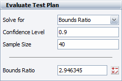
This ratio is analogous to the ratio that can be calculated if a test is conducted and life data are obtained and used to calculate the ratio of the confidence bounds based on the results. Let us use the example in 13.4.3.6 for illustration. For example, if a 90% confidence is desired and 40 units are to be used in the test, then the bounds ratio is calculated as [math]\displaystyle{ 2.9463, }[/math] as shown in Fig. 13.

Fig. 13: Evaluating the test plan using a bounds ratio criterion.

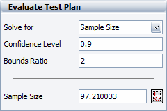
If this calculated bounds ratio is unsatisfactory, the analyst can calculate the required number of units that would meet a certain bounds ratio criterion. For example, if a bounds ratio of 2 is desired, the required sample size is calculated as 97.21, as shown in Fig. 14.

Fig. 14: Evaluation the test plan using a sample size criterion.

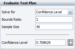
If the sample size is kept at 40 units and a bounds ratio of 2 is desired, the equivalent confidence level we have in the test drops to 70.86%, as shown in Fig. 15.

Fig. 14: Evaluating the test plan using a confidence level criterion.