Optimum Replacement Time Example

New format available! This reference is now available in a new format that offers faster page load, improved display for calculations and images and more targeted search.

As of January 2024, this Reliawiki page will not continue to be updated. Please update all links and bookmarks to the latest references at BlockSim examples and BlockSim reference examples.

---

This example appears in the System analysis reference.

This example demonstrates BlockSim's Optimum Replacement utility, which allows you to determine the most cost-effective time to replace one or more blocks in one or more systems, based on their planned and unplanned replacement costs.

Optimum Replacement Time

The failure distribution of a component is described by a 2-parameter Weibull distribution with [math]\displaystyle{ \beta = 2.5\,\! }[/math] and [math]\displaystyle{ \eta = 1000\,\! }[/math] hours.

• The cost for a corrective replacement is $5.
  
• The cost for a preventive replacement is $1.
  

Estimate the optimum replacement age in order to minimize these costs.

Solution

Prior to obtaining an optimum replacement interval for this component, the assumptions of the following equation must be checked.

[math]\displaystyle{ \begin{align} CPUT\left( t \right)= & \frac{\text{Total Expected Replacement Cost per Cycle}}{\text{Expected Cycle Length}} \\ = & \frac{{{C}_{P}}\cdot R\left( t \right)+{{C}_{U}}\cdot \left[ 1-R\left( t \right) \right]}{\int_{0}^{t}R\left( s \right)ds} \end{align}\,\! }[/math]

The component has an increasing failure rate because it follows a Weibull distribution with [math]\displaystyle{ \beta \,\! }[/math] greater than 1. Note that if [math]\displaystyle{ \beta =1\,\! }[/math], then the component has a constant failure rate, but if [math]\displaystyle{ \beta \lt 1\,\! }[/math], then it has a decreasing failure rate. If either of these cases exist, then preventive replacement is unwise. Furthermore, the cost for preventive replacement is less than the corrective replacement cost. Thus, the conditions for the optimum age replacement policy have been met.

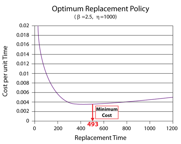
Using BlockSim, enter the parameters of the Weibull distribution in the component's Block Properties window. Next, open the Optimum Replacement window and enter the 1 in the Planned Replacement Cost column, and 5 in the Unplanned Replacement Cost column. Click Calculate. In the Optimum Replacement Calculations window that appears, select the Individual option and click OK. The optimum replacement time for the component is estimated to be 493.0470, as shown next.

The figure below shows the Cost vs. Time plot of the component (with the scaling adjusted and the plot annotated to show the minimum cost).

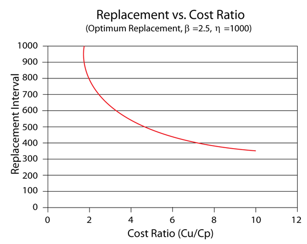
If we enter different cost values in the Unplanned Replacement Cost column and obtain the optimum replacement time at each value, we can use the data points to create a plot that shows the effect of the corrective cost on the optimum replacement interval. The following plot shows an example. In this case, the optimum replacement interval decreases as the cost ratio increases. This is an expected result because the corrective replacement costs are much greater than the preventive replacement costs. Therefore, it is more cost-effective to replace the component more frequently before it fails.