Repairable System Test Design Example - Solve for Time

New format available! This reference is now available in a new format that offers faster page load, improved display for calculations and images and more targeted search.

As of January 2024, this Reliawiki page will not continue to be updated. Please update all links and bookmarks to the latest references at RGA examples and RGA reference examples.

---

This example appears in the Reliability growth reference.

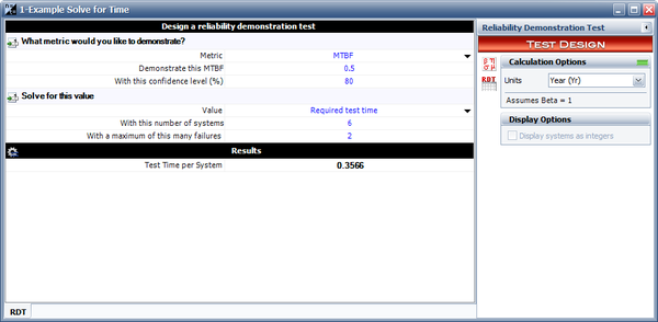
The objective is to design a test to demonstrate that the number of failures per system in five years is less than or equal to 10. In other words, demonstrate that the cumulative MTBF for a repairable system is less than or equal to 0.5 during a five year operating period, with 80% confidence level. Assume that [math]\displaystyle{ \beta =1\,\! }[/math], the number of systems for the test is [math]\displaystyle{ m=6\,\! }[/math] and that the number of allowed failures in the test is [math]\displaystyle{ r=2.\,\! }[/math]

Solution

Since the given requirement is the number of failures, we transfer the requirement to the cumulative MTBF or cumulative failure intensity.

[math]\displaystyle{ MTBF_c=\frac{5}{10}=0.5 year\,\! }[/math]

then:

[math]\displaystyle{ {{\lambda }_{c}}=\frac{1}{MTB{{F}_{c}}}=2\text{ }failures/\ \ year\,\! }[/math]

We can then solve for [math]\displaystyle{ \lambda \,\! }[/math] :

[math]\displaystyle{ {{\lambda }_{c}}\left( t \right)=\lambda {{t}^{\beta -1}}\,\! }[/math]

For the five year period:

[math]\displaystyle{ {{\lambda }_{c}}\left( 5 \right)=\lambda \cdot {{5}^{\beta -1}}\,\! }[/math]

Using the values of [math]\displaystyle{ \lambda \,\! }[/math] and [math]\displaystyle{ \beta \,\! }[/math], we have:

[math]\displaystyle{ 2=\lambda \cdot {{5}^{1-1}}\,\! }[/math]

Then solving for [math]\displaystyle{ \lambda \,\! }[/math] yields:

[math]\displaystyle{ \begin{align} \lambda =2 \end{align}\,\! }[/math]

We can then solve for the required test time, [math]\displaystyle{ T,\,\! }[/math] for each system:

[math]\displaystyle{ 1-CL=\underset{i=0}{\overset{r}{\mathop \sum }}\,\frac{{{\left( m\lambda {{T}^{\beta }} \right)}^{i}}\exp (-m\lambda {{T}^{\beta }})}{i!}\,\! }[/math]

or:

[math]\displaystyle{ 1-0.8=\underset{i=0}{\overset{2}{\mathop \sum }}\,\frac{{{\left( 6\cdot 0.894\cdot {{T}^{1}} \right)}^{i}}\exp (-6\cdot 2\cdot {{T}^{1}})}{i!}\,\! }[/math]

or:

[math]\displaystyle{ \begin{align} 0.2= & exp (-6\cdot 2\cdot T^1) \\ + & \frac{(6\cdot 2\cdot T^1)^1 exp(-6\cdot 2\cdot T^1)}{1!} \\ + & \frac{6\cdot 2\cdot T^1)^2 exp(-6\cdot 2\cdot T^1)}{2!} \\ \end{align}\,\! }[/math]

Solving the above equation numerically yields:

[math]\displaystyle{ T=0.36\,\! }[/math]

In other words, for this example we have to test for 0.36 years to demonstrate that the number of failures per system in five years is less than or equal to 10.

The same result can be obtained in the RGA software, by using the Design of Reliability Tests (DRT) tool. The next figure shows the calculated required test time per system of 0.3566 on the results of the example.