Weibull++ SimuMatic

Reliability analysis using simulation, in which reliability analyses are performed a large number of times on data sets that have been created using Monte Carlo simulation, can be a valuable tool for reliability practitioners. Such simulation analyses can assist the analyst to a) better understand life data analysis concepts, b) experiment with the influences of sample sizes and censoring schemes on analysis methods, c) construct simulation-based confidence intervals, d) better understand the concepts behind confidence intervals and e) design reliability tests. This section explores some of the results that can be obtained from simulation analyses using the Weibull++ SimuMatic tool.

Parameter Estimation and Confidence Bounds Techniques

In life data analysis, we use data (usually times-to-failure or times-to-success data) obtained from a sample of units to make predictions for the entire population of units. Depending on the sample size, the data censoring scheme and the parameter estimation method, the amount of error in the results can vary widely. To quantify this sampling error, or uncertainty, confidence bounds are widely used. In addition to the analytical calculation methods that are available, simulation can also be used. SimuMatic generates these confidence bounds and assists the practitioner (or the teacher) to visualize and understand them. In addition, it allows the analyst to determine the adequacy of certain parameter estimation methods (such as rank regression on X, rank regression on Y and maximum likelihood estimation) and to visualize the effects of different data censoring schemes on the confidence bounds.

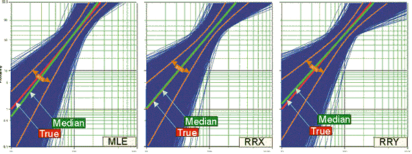
As an example, we will attempt to determine the best parameter estimation method for a sample of ten units following a Weibull distribution with [math]\displaystyle{ \beta = 2\,\! }[/math] and [math]\displaystyle{ \eta = 100\,\! }[/math] and with complete time-to-failure data for each unit (i.e., no censoring). Using SimuMatic, 10,000 data sets are generated (using Monte Carlo methods based on the Weibull distribution) and we estimate their parameters using RRX, RRY and MLE. The plotted results generated by SimuMatic are shown next.

The results clearly demonstrate that the median RRX estimate provides the least deviation from the truth for this sample size and data type. However, the MLE outputs are grouped more closely together, as evidenced by the confidence bounds. The same figures also show the simulation-based bounds, as well as the expected variation due to sampling error.

This experiment can be repeated in SimuMatic using multiple censoring schemes (including Type I and Type II right censoring as well as random censoring) with the included distributions. We can perform multiple experiments with this utility to evaluate our assumptions about the appropriate parameter estimation method to use for the data set.

Using Simulation to Design Reliability Tests

Good reliability specifications include requirements for reliability and an associated lower one-sided confidence interval. When designing a test, we must determine the sample size to test as well as the expected test duration. The next simple example illustrates the methods available in SimuMatic.

Let us assume that a specific reliability specification states that at T=10 hr the reliability must be 99%, or R(T=10)=99% (unreliability = 1%), and at T=20 hr the reliability must be 90%, or R(T=20)=90%, at an 80% lower one-sided confidence level ( L1S=80% ).

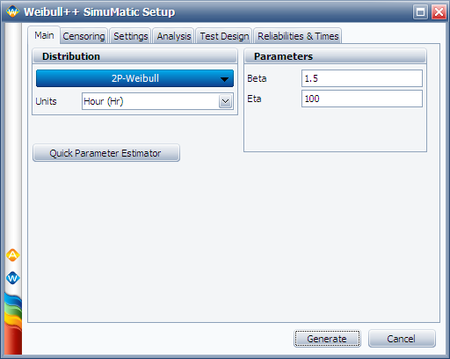
One way to meet this specification is to design a test that will demonstrate either of these requirements at L1S=80% with the required parameters (for this example we will use the R(T=10)=99% @ L1S=80% requirement). With SimuMatic, we can specify the underlying distribution, distribution parameters (the Quick Parameter Estimator tool can be utilized), sample size on test, censoring scheme, required reliability and associated confidence level. From these inputs, SimuMatic will solve (via simulation) for the time demonstrated at the specified reliability and confidence level (i.e., X in the R(T=X)=99% @ L1S=80% formulation), as well as the expected test duration. If the demonstrated time is greater than the time requirement, this indicates that the test design would accomplish its required objective. Since there are multiple test designs that may accomplish the objective, multiple experiments should be performed until we arrive at an acceptable test design (i.e., number of units and test duration).

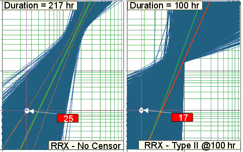
We start with a test design using a sample size of ten, with no censoring (i.e., all units to be tested to failure). We perform the analysis using RRX and 10,000 simulated data sets. The outcome is an expected test duration of 217 hr and a demonstrated time of 25 hr. This result is well above the stated requirement of 10 hr (note that in this case, the true value of T at a 50% CL, for R = 99%, is 40 hrs which gives us a ratio of 1.6 between true and demonstrated). Since this would demonstrate the requirement, we can then attempt to reduce the number of units or test time. Suppose that we need to bring the test time down to 100 hr (instead of the expected 217 hr). The test could then be designed using Type II censoring (i.e., any unit that has not failed by 100 hr is right censored) assuring completion by 100 hr. Again, we specify Type II censoring at 100 hr in SimuMatic, and we repeat the simulation with the same parameters as before. The simulation results in this case yield an expected test duration of 100 hr and a demonstrated time of 17 hr at the stated requirements. This result is also above our requirement The next figure graphically shows the results of this experiment. This process can then be repeated using different sample sizes and censoring schemes until we arrive at a desirable test plan.