Normal Parameter Estimation
Estimation of the Parameters
Probability Plotting
As described before, probability plotting involves plotting the failure times and associated unreliability estimates on specially constructed probability plotting paper. The form of this paper is based on a linearization of the cdf of the specific distribution. For the normal distribution, the cumulative density function can be written as:
- [math]\displaystyle{ F(t)=\Phi \left( \frac{t-\mu }{{{\sigma }}} \right)\,\! }[/math]
or:
- [math]\displaystyle{ {{\Phi }^{-1}}\left[ F(t) \right]=-\frac{\mu}{\sigma}+\frac{1}{\sigma}t\,\! }[/math]
where:
- [math]\displaystyle{ \Phi (x)=\frac{1}{\sqrt{2\pi }}\int_{-\infty }^{x}{{e}^{-\tfrac{{{t}^{2}}}{2}}}dt\,\! }[/math]
Now, let:
- [math]\displaystyle{ y={{\Phi }^{-1}}\left[ F(t) \right]\,\! }[/math]
- [math]\displaystyle{ a=-\frac{\mu }{\sigma }\,\! }[/math]
and:
- [math]\displaystyle{ b=\frac{1}{\sigma }\,\! }[/math]
which results in the linear equation of:
- [math]\displaystyle{ \begin{align} y=a+bt \end{align}\,\! }[/math]
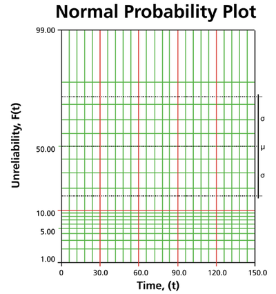
The normal probability paper resulting from this linearized cdf function is shown next.
Since the normal distribution is symmetrical, the area under the pdf curve from [math]\displaystyle{ -\infty \,\! }[/math] to [math]\displaystyle{ \mu \,\! }[/math] is [math]\displaystyle{ 0.5\,\! }[/math], as is the area from [math]\displaystyle{ \mu \,\! }[/math] to [math]\displaystyle{ +\infty \,\! }[/math]. Consequently, the value of [math]\displaystyle{ \mu \,\! }[/math] is said to be the point where [math]\displaystyle{ R(t)=Q(t)=50%\,\! }[/math]. This means that the estimate of [math]\displaystyle{ \mu \,\! }[/math] can be read from the point where the plotted line crosses the 50% unreliability line.
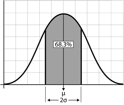
To determine the value of [math]\displaystyle{ \sigma \,\! }[/math] from the probability plot, it is first necessary to understand that the area under the pdf curve that lies between one standard deviation in either direction from the mean (or two standard deviations total) represents 68.3% of the area under the curve. This is represented graphically in the following figure.
Consequently, the interval between [math]\displaystyle{ Q(t)=84.15%\,\! }[/math] and [math]\displaystyle{ Q(t)=15.85%\,\! }[/math] represents two standard deviations, since this is an interval of 68.3% ( [math]\displaystyle{ 84.15-15.85=68.3\,\! }[/math] ), and is centered on the mean at 50%. As a result, the standard deviation can be estimated from:
- [math]\displaystyle{ \widehat{\sigma }=\frac{t(Q=84.15%)-t(Q=15.85%)}{2}\,\! }[/math]
That is: the value of [math]\displaystyle{ \widehat{\sigma }\,\! }[/math] is obtained by subtracting the time value where the plotted line crosses the 84.15% unreliability line from the time value where the plotted line crosses the 15.85% unreliability line and dividing the result by two. This process is illustrated in the following example.
Normal Distribution Probability Plotting Example
7 units are put on a life test and run until failure. The failure times are 85, 90, 95, 100, 105, 110, and 115 hours. Assuming a normal distribution, estimate the parameters using probability plotting.
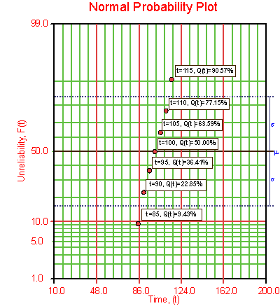
In order to plot the points for the probability plot, the appropriate estimates for the unreliability values must be obtained. These values will be estimated through the use of median ranks, which can be obtained from statistical tables or from the Quick Statistical Reference (QSR) tool in Weibull++. The following table shows the times-to-failure and the appropriate median rank values for this example:
These points can now be plotted on a normal probability plotting paper as shown in the next figure.
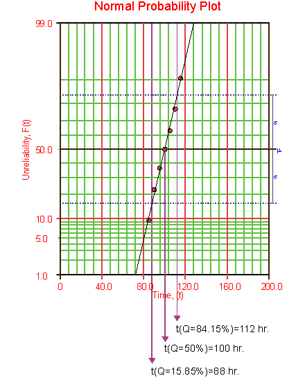
Draw the best possible line through the plot points. The time values where the line intersects the 15.85%, 50%, and 84.15% unreliability values should be projected down to the abscissa, as shown in the following plot.
The estimate of [math]\displaystyle{ \mu \,\! }[/math] is determined from the time value at the 50% unreliability level, which in this case is 100 hours. The value of the estimator of [math]\displaystyle{ \sigma \,\! }[/math] is determined as follows:
- [math]\displaystyle{ \begin{align} \widehat{\sigma }= & \frac{t(Q=84.15%)-t(Q=15.85%)}{2} \\ \widehat{\sigma }= & \frac{112-88}{2}=\frac{24}{2} \\ \widehat{\sigma }= & 12\text{ hours} \end{align}\,\! }[/math]
Alternately, [math]\displaystyle{ \widehat{\sigma }\,\! }[/math] could be determined by measuring the distance from [math]\displaystyle{ t(Q=15.85%)\,\! }[/math] to [math]\displaystyle{ t(Q=50%)\,\! }[/math], or [math]\displaystyle{ t(Q=50%)\,\! }[/math] to [math]\displaystyle{ t(Q=84.15%)\,\! }[/math], as either of these two distances is equal to the value of one standard deviation.
Rank Regression on Y
Performing rank regression on Y requires that a straight line be fitted to a set of data points such that the sum of the squares of the vertical deviations from the points to the line is minimized.
The least squares parameter estimation method (regression analysis) was discussed in Parameter Estimation, and the following equations for regression on Y were derived:
- [math]\displaystyle{ \begin{align}\hat{a}= & \bar{b}-\hat{b}\bar{x} \\ =& \frac{\sum_{i=1}^N y_{i}}{N}-\hat{b}\frac{\sum_{i=1}^{N}x_{i}}{N}\\ \end{align} \,\! }[/math]
and:
- [math]\displaystyle{ \hat{b}=\frac{\underset{i=1}{\overset{N}{\mathop{\sum }}}\,{{x}_{i}}{{y}_{i}}-\tfrac{\underset{i=1}{\overset{N}{\mathop{\sum }}}\,{{x}_{i}}\underset{i=1}{\overset{N}{\mathop{\sum }}}\,{{y}_{i}}}{N}}{\underset{i=1}{\overset{N}{\mathop{\sum }}}\,x_{i}^{2}-\tfrac{{{\left( \underset{i=1}{\overset{N}{\mathop{\sum }}}\,{{x}_{i}} \right)}^{2}}}{N}}\,\! }[/math]
In the case of the normal distribution, the equations for [math]\displaystyle{ {{y}_{i}}\,\! }[/math] and [math]\displaystyle{ {{x}_{i}}\,\! }[/math] are:
- [math]\displaystyle{ {{y}_{i}}={{\Phi }^{-1}}\left[ F({{t}_{i}}) \right]\,\! }[/math]
and:
- [math]\displaystyle{ \begin{align} {{x}_{i}}={{t}_{i}} \end{align}\,\! }[/math]
where the values for [math]\displaystyle{ F({{T}_{i}})\,\! }[/math] are estimated from the median ranks. Once [math]\displaystyle{ \widehat{a}\,\! }[/math] and [math]\displaystyle{ \widehat{b}\,\! }[/math] are obtained, [math]\displaystyle{ \widehat{\sigma }\,\! }[/math] and [math]\displaystyle{ \widehat{\mu }\,\! }[/math] can easily be obtained from above equations.
The Correlation Coefficient
The estimator of the sample correlation coefficient, [math]\displaystyle{ \hat{\rho }\,\! }[/math], is given by:
- [math]\displaystyle{ \hat{\rho }=\frac{\underset{i=1}{\overset{N}{\mathop{\sum }}}\,({{x}_{i}}-\overline{x})({{y}_{i}}-\overline{y})}{\sqrt{\underset{i=1}{\overset{N}{\mathop{\sum }}}\,{{({{x}_{i}}-\overline{x})}^{2}}\cdot \underset{i=1}{\overset{N}{\mathop{\sum }}}\,{{({{y}_{i}}-\overline{y})}^{2}}}}\,\! }[/math]
RRY Example
Normal Distribution RRY Example
14 units were reliability tested and the following life test data were obtained. Assuming the data follow a normal distribution, estimate the parameters and determine the correlation coefficient, [math]\displaystyle{ \rho\,\! }[/math], using rank regression on Y.
| The test data | |
|---|---|
| Data point index | Time-to-failure |
| 1 | 5 |
| 2 | 10 |
| 3 | 15 |
| 4 | 20 |
| 5 | 25 |
| 6 | 30 |
| 7 | 35 |
| 8 | 40 |
| 9 | 50 |
| 10 | 60 |
| 11 | 70 |
| 12 | 80 |
| 13 | 90 |
| 14 | 100 |
Solution
Construct a table like the one shown next.
- The median rank values ( [math]\displaystyle{ F({{t}_{i}})\,\! }[/math] ) can be found in rank tables, available in many statistical texts, or they can be estimated by using the Quick Statistical Reference in Weibull++.
- The [math]\displaystyle{ {{y}_{i}}\,\! }[/math] values were obtained from standardized normal distribution's area tables by entering for [math]\displaystyle{ F(z)\,\! }[/math] and getting the corresponding [math]\displaystyle{ z\,\! }[/math] value ( [math]\displaystyle{ {{y}_{i}}\,\! }[/math] ). As with the median rank values, these standard normal values can be obtained with the Quick Statistical Reference.
Given the values in the table above, calculate [math]\displaystyle{ \widehat{a}\,\! }[/math] and [math]\displaystyle{ \widehat{b}\,\! }[/math] using:
- [math]\displaystyle{ \begin{align} & \widehat{b}= & \frac{\underset{i=1}{\overset{14}{\mathop{\sum }}}\,{{T}_{i}}{{y}_{i}}-(\underset{i=1}{\overset{14}{\mathop{\sum }}}\,{{T}_{i}})(\underset{i=1}{\overset{14}{\mathop{\sum }}}\,{{y}_{i}})/14}{\underset{i=1}{\overset{14}{\mathop{\sum }}}\,T_{i}^{2}-{{(\underset{i=1}{\overset{14}{\mathop{\sum }}}\,{{T}_{i}})}^{2}}/14} \\ & & \\ & \widehat{b}= & \frac{365.2711-(630)(0)/14}{40,600-{{(630)}^{2}}/14}=0.02982 \end{align}\,\! }[/math]
and:
- [math]\displaystyle{ \widehat{a}=\overline{y}-\widehat{b}\overline{T}=\frac{\underset{i=1}{\overset{N}{\mathop{\sum }}}\,{{y}_{i}}}{N}-\widehat{b}\frac{\underset{i=1}{\overset{N}{\mathop{\sum }}}\,{{t}_{i}}}{N}\,\! }[/math]
or:
- [math]\displaystyle{ \widehat{a}=\frac{0}{14}-(0.02982)\frac{630}{14}=-1.3419\,\! }[/math]
Therefore:
- [math]\displaystyle{ \widehat{\sigma}=\frac{1}{\hat{b}}=\frac{1}{0.02982}=33.5367\,\! }[/math]
and:
- [math]\displaystyle{ \widehat{\mu }=-\widehat{a}\cdot \widehat{\sigma }=-(-1.3419)\cdot 33.5367\simeq 45\,\! }[/math]
or [math]\displaystyle{ \widehat{\mu }=45\,\! }[/math] hours [math]\displaystyle{ .\,\! }[/math]
The correlation coefficient can be estimated using:
- [math]\displaystyle{ \widehat{\rho }=0.979\,\! }[/math]
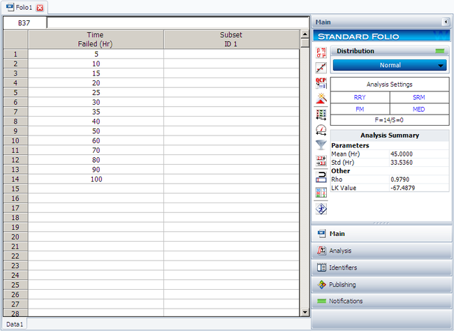
The preceding example can be repeated using Weibull++ .
- Create a new folio for Times-to-Failure data, and enter the data given in this example.
- Choose Normal from the Distributions list.
- Go to the Analysis page and select Rank Regression on Y (RRY).
- Click the Calculate icon located on the Main page.
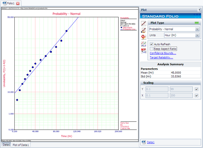
The probability plot is shown next.
Rank Regression on X
As was mentioned previously, performing a rank regression on X requires that a straight line be fitted to a set of data points such that the sum of the squares of the horizontal deviations from the points to the fitted line is minimized.
Again, the first task is to bring our function, the probability of failure function for normal distribution, into a linear form. This step is exactly the same as in regression on Y analysis. All other equations apply in this case as they did for the regression on Y. The deviation from the previous analysis begins on the least squares fit step where: in this case, we treat [math]\displaystyle{ x\,\! }[/math] as the dependent variable and [math]\displaystyle{ y\,\! }[/math] as the independent variable. The best-fitting straight line for the data, for regression on X, is the straight line:
- [math]\displaystyle{ x=\widehat{a}+\widehat{b}y\,\! }[/math]
The corresponding equations for [math]\displaystyle{ \widehat{a}\,\! }[/math] and [math]\displaystyle{ \widehat{b}\,\! }[/math] are:
- [math]\displaystyle{ \hat{a}=\overline{x}-\hat{b}\overline{y}=\frac{\underset{i=1}{\overset{N}{\mathop{\sum }}}\,{{x}_{i}}}{N}-\hat{b}\frac{\underset{i=1}{\overset{N}{\mathop{\sum }}}\,{{y}_{i}}}{N}\,\! }[/math]
and:
- [math]\displaystyle{ \hat{b}=\frac{\underset{i=1}{\overset{N}{\mathop{\sum }}}\,{{x}_{i}}{{y}_{i}}-\tfrac{\underset{i=1}{\overset{N}{\mathop{\sum }}}\,{{x}_{i}}\underset{i=1}{\overset{N}{\mathop{\sum }}}\,{{y}_{i}}}{N}}{\underset{i=1}{\overset{N}{\mathop{\sum }}}\,y_{i}^{2}-\tfrac{{{\left( \underset{i=1}{\overset{N}{\mathop{\sum }}}\,{{y}_{i}} \right)}^{2}}}{N}}\,\! }[/math]
where:
- [math]\displaystyle{ {{y}_{i}}={{\Phi }^{-1}}\left[ F({{t}_{i}}) \right]\,\! }[/math]
and:
- [math]\displaystyle{ \begin{align} {{x}_{i}}={{t}_{i}} \end{align}\,\! }[/math]
and the [math]\displaystyle{ F({{t}_{i}})\,\! }[/math] values are estimated from the median ranks. Once [math]\displaystyle{ \widehat{a}\,\! }[/math] and [math]\displaystyle{ \widehat{b}\,\! }[/math] are obtained, solve the above linear equation for the unknown value of [math]\displaystyle{ y\,\! }[/math] which corresponds to:
- [math]\displaystyle{ y=-\frac{\widehat{a}}{\widehat{b}}+\frac{1}{\widehat{b}}x\,\! }[/math]
Solving for the parameters, we get:
- [math]\displaystyle{ a=-\frac{\widehat{a}}{\widehat{b}}=-\frac{\mu }{\sigma }\Rightarrow \mu =\widehat{a}\,\! }[/math]
and:
- [math]\displaystyle{ b=\frac{1}{\widehat{b}}=\frac{1}{\sigma }\Rightarrow \sigma =\widehat{b}\,\! }[/math]
The correlation coefficient is evaluated as before.
RRX Example
Normal Distribution RRX Example
Using the same data set from the RRY example given above, and assuming a normal distribution, estimate the parameters and determine the correlation coefficient, [math]\displaystyle{ \rho \,\! }[/math], using rank regression on X.
Solution
The table constructed for the RRY analysis applies to this example also. Using the values on this table, we get:
- [math]\displaystyle{ \begin{align} \hat{b}= & \frac{\underset{i=1}{\overset{14}{\mathop{\sum }}}\,{{t}_{i}}{{y}_{i}}-\tfrac{\underset{i=1}{\overset{14}{\mathop{\sum }}}\,{{t}_{i}}\underset{i=1}{\overset{14}{\mathop{\sum }}}\,{{y}_{i}}}{14}}{\underset{i=1}{\overset{14}{\mathop{\sum }}}\,y_{i}^{2}-\tfrac{{{\left( \underset{i=1}{\overset{14}{\mathop{\sum }}}\,{{y}_{i}} \right)}^{2}}}{14}} \\ \widehat{b}= & \frac{365.2711-(630)(0)/14}{11.3646-{{(0)}^{2}}/14}=32.1411 \end{align}\,\! }[/math]
and:
- [math]\displaystyle{ \hat{a}=\overline{x}-\hat{b}\overline{y}=\frac{\underset{i=1}{\overset{14}{\mathop{\sum }}}\,{{t}_{i}}}{14}-\widehat{b}\frac{\underset{i=1}{\overset{14}{\mathop{\sum }}}\,{{y}_{i}}}{14}\,\! }[/math]
or:
- [math]\displaystyle{ \widehat{a}=\frac{630}{14}-(32.1411)\frac{(0)}{14}=45\,\! }[/math]
Therefore:
- [math]\displaystyle{ \widehat{\sigma }=\widehat{b}=32.1411\,\! }[/math]
and:
- [math]\displaystyle{ \widehat{\mu }=\widehat{a}=45\text{ hours}\,\! }[/math]
The correlation coefficient is obtained as:
- [math]\displaystyle{ \widehat{\rho }=0.979\,\! }[/math]
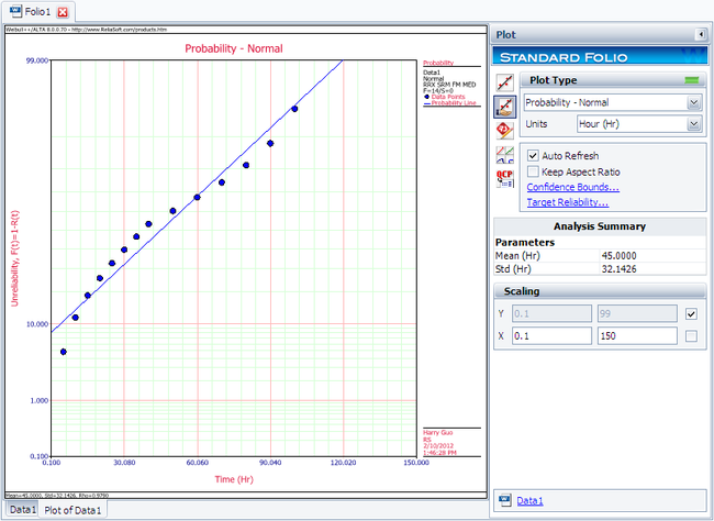
Note that the results for regression on X are not necessarily the same as the results for regression on Y. The only time when the two regressions are the same (i.e., will yield the same equation for a line) is when the data lie perfectly on a straight line.
The plot of the Weibull++ solution for this example is shown next.
Maximum Likelihood Estimation
As it was outlined in Parameter Estimation, maximum likelihood estimation works by developing a likelihood function based on the available data and finding the values of the parameter estimates that maximize the likelihood function. This can be achieved by using iterative methods to determine the parameter estimate values that maximize the likelihood function. This can be rather difficult and time-consuming, particularly when dealing with the three-parameter distribution. Another method of finding the parameter estimates involves taking the partial derivatives of the likelihood function with respect to the parameters, setting the resulting equations equal to zero, and solving simultaneously to determine the values of the parameter estimates. The log-likelihood functions and associated partial derivatives used to determine maximum likelihood estimates for the normal distribution are covered in the Appendix.
Special Note About Bias
Estimators (i.e., parameter estimates) have properties such as unbiasedness, minimum variance, sufficiency, consistency, squared error constancy, efficiency and completeness, as discussed in Dudewicz and Mishra [7] and in Dietrich [5]. Numerous books and papers deal with these properties and this coverage is beyond the scope of this reference.
However, we would like to briefly address one of these properties, unbiasedness. An estimator is said to be unbiased if the estimator [math]\displaystyle{ \widehat{\theta }=d({{X}_{1,}}{{X}_{2,}}...,{{X}_{n)}}\,\! }[/math] satisfies the condition [math]\displaystyle{ E\left[ \widehat{\theta } \right]\,\! }[/math] [math]\displaystyle{ =\theta \,\! }[/math] for all [math]\displaystyle{ \theta \in \Omega .\,\! }[/math]
Note that [math]\displaystyle{ E\left[ X \right]\,\! }[/math] denotes the expected value of X and is defined (for continuous distributions) by:
- [math]\displaystyle{ \begin{align} E\left[ X \right]= \int_{\varpi }x\cdot f(x)dx \\ X\in & \varpi . \end{align}\,\! }[/math]
It can be shown in Dudewicz and Mishra [7] and in Dietrich [5] that the MLE estimator for the mean of the normal (and lognormal) distribution does satisfy the unbiasedness criteria, or [math]\displaystyle{ E\left[ \widehat{\mu } \right]\,\! }[/math] [math]\displaystyle{ =\mu .\,\! }[/math] The same is not true for the estimate of the variance [math]\displaystyle{ \hat{\sigma }^{2}\,\! }[/math]. The maximum likelihood estimate for the variance for the normal distribution is given by:
- [math]\displaystyle{ \hat{\sigma }^{2}=\frac{1}{N}\underset{i=1}{\overset{N}{\mathop \sum }}\,{{({{t}_{i}}-\bar{T})}^{2}}\,\! }[/math]
with a standard deviation of:
- [math]\displaystyle{ {{\hat{\sigma }}}=\sqrt{\frac{1}{N}\underset{i=1}{\overset{N}{\mathop \sum }}\,{{({{t}_{i}}-\bar{T})}^{2}}}\,\! }[/math]
These estimates, however, have been shown to be biased. It can be shown in Dudewicz and Mishra [7] and in Dietrich [5] that the unbiased estimate of the variance and standard deviation for complete data is given by:
- [math]\displaystyle{ \begin{align} \hat{\sigma }^{2}= & \left[ \frac{N}{N-1} \right]\cdot \left[ \frac{1}{N}\underset{i=1}{\overset{N}{\mathop \sum }}\,{{({{t}_{i}}-\bar{T})}^{2}} \right]=\frac{1}{N-1}\underset{i=1}{\overset{N}{\mathop \sum }}\,{{({{t}_{i}}-\bar{T})}^{2}} \\ {{{\hat{\sigma }}}}= & \sqrt{\left[ \frac{N}{N-1} \right]\cdot \left[ \frac{1}{N}\underset{i=1}{\overset{N}{\mathop \sum }}\,{{({{t}_{i}}-\bar{T})}^{2}} \right]} \\ = & \sqrt{\frac{1}{N-1}\underset{i=1}{\overset{N}{\mathop \sum }}\,{{({{t}_{i}}-\bar{T})}^{2}}} \end{align}\,\! }[/math]
Note that for larger values of [math]\displaystyle{ N\,\! }[/math], [math]\displaystyle{ \sqrt{\left[ N/(N-1) \right]}\,\! }[/math] tends to 1.
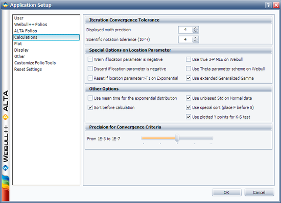
The Use Unbiased Std on Normal Data option on the Calculations page of the User Setup allows biasing to be considered when estimating the parameters.
When this option is selected, Weibull++ returns the unbiased standard deviation as defined. This is only true for complete data sets. For all other data types, Weibull++ by default returns the biased standard deviation as defined above regardless of the selection status of this option. The next figure shows this setting in Weibull++.
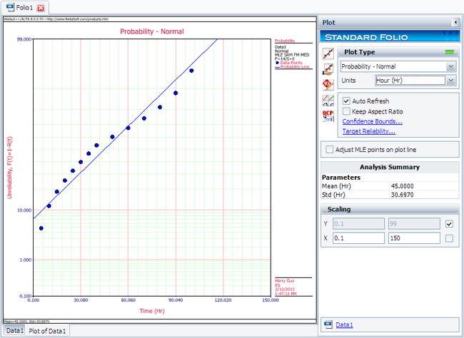
MLE Example
Normal Distribution MLE Example
Using the same data set from the RRY and RRX examples given above and assuming a normal distribution, estimate the parameters using the MLE method.
Solution
In this example we have non-grouped data without suspensions and without interval data. The partial derivatives of the normal log-likelihood function, [math]\displaystyle{ \Lambda ,\,\! }[/math] are given by:
- [math]\displaystyle{ \begin{align} \frac{\partial \Lambda }{\partial \mu }= & \frac{1}{{{\sigma }^{2}}}\underset{i=1}{\overset{14}{\mathop \sum }}\,({{t}_{i}}-\mu )=0 \\ \frac{\partial \Lambda }{\partial \sigma }= & \underset{i=1}{\overset{14}{\mathop \sum }}\,\left( \frac{{{t}_{i}}-\mu }{{{\sigma }^{3}}}-\frac{1}{\sigma } \right)=0 \end{align}\,\! }[/math]
(The derivations of these equations are presented in the appendix.) Substituting the values of [math]\displaystyle{ {{t}_{i}}\,\! }[/math] and solving the above system simultaneously, we get [math]\displaystyle{ \widehat{\sigma }=29.58\,\! }[/math] hours [math]\displaystyle{ ,\,\! }[/math] [math]\displaystyle{ \widehat{\mu }=45\,\! }[/math] hours [math]\displaystyle{ .\,\! }[/math]
The Fisher matrix is:
- [math]\displaystyle{ \left[ \begin{matrix} \widehat{Var}\left( \widehat{\mu } \right)=62.5000 & {} & \widehat{Cov}\left( \widehat{\mu },\widehat{\sigma } \right)=0.0000 \\ {} & {} & {} \\ \widehat{Cov}\left( \widehat{\mu },\widehat{\sigma } \right)=0.0000 & {} & \widehat{Var}\left( \widehat{\sigma } \right)=31.2500 \\ \end{matrix} \right]\,\! }[/math]
The plot of the Weibull++ solution for this example is shown next.

