Exponential Parameter Estimation

Estimation of the Exponential Parameters

Probability Plotting

Estimation of the parameters for the exponential distribution via probability plotting is very similar to the process used when dealing with the Weibull distribution. Recall, however, that the appearance of the probability plotting paper and the methods by which the parameters are estimated vary from distribution to distribution, so there will be some noticeable differences. In fact, due to the nature of the exponential cdf, the exponential probability plot is the only one with a negative slope. This is because the y-axis of the exponential probability plotting paper represents the reliability, whereas the y-axis for most of the other life distributions represents the unreliability.

This is illustrated in the process of linearizing the cdf, which is necessary to construct the exponential probability plotting paper. For the two-parameter exponential distribution the cumulative density function is given by:

[math]\displaystyle{ \begin{align} F(t)=1-{{e}^{-\lambda (t-\gamma )}} \end{align}\,\! }[/math]

Taking the natural logarithm of both sides of the above equation yields:

[math]\displaystyle{ \ln \left[ 1-F(t) \right]=-\lambda (t-\gamma )\,\! }[/math]

or:

[math]\displaystyle{ \begin{align} \ln [1-F(t)]=\lambda \gamma -\lambda t \end{align}\,\! }[/math]

Now, let:

[math]\displaystyle{ \begin{align} y=\ln [1-F(t)] \end{align}\,\! }[/math]

[math]\displaystyle{ \begin{align} a=\lambda \gamma \end{align}\,\! }[/math]

and:

[math]\displaystyle{ \begin{align} b=-\lambda \end{align}\,\! }[/math]

which results in the linear equation of:

[math]\displaystyle{ \begin{align} y=a+bt \end{align}\,\! }[/math]

Note that with the exponential probability plotting paper, the y-axis scale is logarithmic and the x-axis scale is linear. This means that the zero value is present only on the x-axis. For [math]\displaystyle{ t=0\,\! }[/math], [math]\displaystyle{ R=1\,\! }[/math] and [math]\displaystyle{ F(t)=0\,\! }[/math]. So if we were to use [math]\displaystyle{ F(t)\,\! }[/math] for the y-axis, we would have to plot the point [math]\displaystyle{ (0,0)\,\! }[/math]. However, since the y-axis is logarithmic, there is no place to plot this on the exponential paper. Also, the failure rate, [math]\displaystyle{ \lambda \,\! }[/math], is the negative of the slope of the line, but there is an easier way to determine the value of [math]\displaystyle{ \lambda \,\! }[/math] from the probability plot, as will be illustrated in the following example.

Plotting Example

1-Parameter Exponential Probability Plot Example

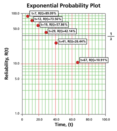
6 units are put on a life test and tested to failure. The failure times are 7, 12, 19, 29, 41, and 67 hours. Estimate the failure rate for a 1-parameter exponential distribution using the probability plotting method.

In order to plot the points for the probability plot, the appropriate reliability estimate values must be obtained. These will be equivalent to [math]\displaystyle{ 100%-MR\,\! }[/math] since the y-axis represents the reliability and the [math]\displaystyle{ MR\,\! }[/math] values represent unreliability estimates.

[math]\displaystyle{ \begin{matrix} \text{Time-to-failure, hr} & \text{Reliability Estimate, }% \\ 7 & 100-10.91=89.09% \\ 12 & 100-26.44=73.56% \\ 19 & 100-42.14=57.86% \\ 29 & 100-57.86=42.14% \\ 41 & 100-73.56=26.44% \\ 67 & 100-89.09=10.91% \\ \end{matrix}\,\! }[/math]

Next, these points are plotted on an exponential probability plotting paper. A sample of this type of plotting paper is shown next, with the sample points in place. Notice how these points describe a line with a negative slope.

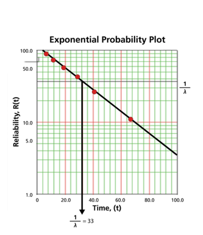
Once the points are plotted, draw the best possible straight line through these points. The time value at which this line intersects with a horizontal line drawn at the 36.8% reliability mark is the mean life, and the reciprocal of this is the failure rate [math]\displaystyle{ \lambda\,\! }[/math]. This is because at [math]\displaystyle{ t=m=\tfrac{1}{\lambda }\,\! }[/math]:

[math]\displaystyle{ \begin{align} R(t)= & {{e}^{-\lambda \cdot t}} \\ R(t)= & {{e}^{-\lambda \cdot \tfrac{1}{\lambda }}} \\ R(t)= & {{e}^{-1}}=0.368=36.8%. \end{align}\,\! }[/math]

The following plot shows that the best-fit line through the data points crosses the [math]\displaystyle{ R=36.8%\,\! }[/math] line at [math]\displaystyle{ t=33\,\! }[/math] hours. And because [math]\displaystyle{ \tfrac{1}{\lambda }=33\,\! }[/math] hours, [math]\displaystyle{ \lambda =0.0303\,\! }[/math] failures/hour.

Rank Regression on Y

Performing a rank regression on Y requires that a straight line be fitted to the set of available data points such that the sum of the squares of the vertical deviations from the points to the line is minimized. The least squares parameter estimation method (regression analysis) was discussed in Parameter Estimation, and the following equations for rank regression on Y (RRY) were derived:

[math]\displaystyle{ \hat{a}=\bar{y}-\hat{b}\bar{x}=\frac{\underset{i=1}{\overset{N}{\mathop{\sum }}}\,{{y}_{i}}}{N}-\hat{b}\frac{\underset{i=1}{\overset{N}{\mathop{\sum }}}\,{{x}_{i}}}{N}\,\! }[/math]

and:

[math]\displaystyle{ \hat{b}=\frac{\underset{i=1}{\overset{N}{\mathop{\sum }}}\,{{x}_{i}}{{y}_{i}}-\tfrac{\underset{i=1}{\overset{N}{\mathop{\sum }}}\,{{x}_{i}}\underset{i=1}{\overset{N}{\mathop{\sum }}}\,{{y}_{i}}}{N}}{\underset{i=1}{\overset{N}{\mathop{\sum }}}\,x_{i}^{2}-\tfrac{{{\left( \underset{i=1}{\overset{N}{\mathop{\sum }}}\,{{x}_{i}} \right)}^{2}}}{N}}\,\! }[/math]

In our case, the equations for [math]\displaystyle{ {{y}_{i}}\,\! }[/math] and [math]\displaystyle{ {{x}_{i}}\,\! }[/math] are:

[math]\displaystyle{ \begin{align} {{y}_{i}}=\ln [1-F({{t}_{i}})] \end{align}\,\! }[/math]

and:

[math]\displaystyle{ \begin{align} {{x}_{i}}={{t}_{i}} \end{align}\,\! }[/math]

and the [math]\displaystyle{ F({{t}_{i}})\,\! }[/math] is estimated from the median ranks. Once [math]\displaystyle{ \hat{a}\,\! }[/math] and [math]\displaystyle{ \hat{b}\,\! }[/math] are obtained, then [math]\displaystyle{ \hat{\lambda }\,\! }[/math] and [math]\displaystyle{ \hat{\gamma }\,\! }[/math] can easily be obtained from above equations. For the one-parameter exponential, equations for estimating a and b become:

[math]\displaystyle{ \begin{align} \hat{a}= & 0, \\ \hat{b}= & \frac{\underset{i=1}{\overset{N}{\mathop{\sum }}}\,{{x}_{i}}{{y}_{i}}}{\underset{i=1}{\overset{N}{\mathop{\sum }}}\,x_{i}^{2}} \end{align}\,\! }[/math]

The Correlation Coefficient

The estimator of [math]\displaystyle{ \rho \,\! }[/math] is the sample correlation coefficient, [math]\displaystyle{ \hat{\rho }\,\! }[/math], given by:

[math]\displaystyle{ \hat{\rho }=\frac{\underset{i=1}{\overset{N}{\mathop{\sum }}}\,({{x}_{i}}-\overline{x})({{y}_{i}}-\overline{y})}{\sqrt{\underset{i=1}{\overset{N}{\mathop{\sum }}}\,{{({{x}_{i}}-\overline{x})}^{2}}\cdot \underset{i=1}{\overset{N}{\mathop{\sum }}}\,{{({{y}_{i}}-\overline{y})}^{2}}}}\,\! }[/math]

RRY Example

2-Parameter Exponential RRY Example
14 units were being reliability tested and the following life test data were obtained. Assuming that the data follow a 2-parameter exponential distribution, estimate the parameters and determine the correlation coefficient, [math]\displaystyle{ \rho \,\! }[/math], using rank regression on Y (RRY).

Life Test Data
Data point index	Time-to-failure
1	5
2	10
3	15
4	20
5	25
6	30
7	35
8	40
9	50
10	60
11	70
12	80
13	90
14	100

Solution

Construct the following table, as shown next.

[math]\displaystyle{ \overset{{}}{\mathop{\text{Table}\text{- Least Squares Analysis}}}\,\,\! }[/math] [math]\displaystyle{ \begin{matrix} N & t_{i} & F(t_{i}) & y_{i} & t_{i}^{2} & y_{i}^{2} & t_{i} y_{i} \\ \text{1} & \text{5} & \text{0}\text{.0483} & \text{-0}\text{.0495} & \text{25} & \text{0}\text{.0025} & \text{-0}\text{.2475} \\ \text{2} & \text{10} & \text{0}\text{.1170} & \text{-0}\text{.1244} & \text{100} & \text{0}\text{.0155} & \text{-1}\text{.2443} \\ \text{3} & \text{15} & \text{0}\text{.1865} & \text{-0}\text{.2064} & \text{225} & \text{0}\text{.0426} & \text{-3}\text{.0961} \\ \text{4} & \text{20} & \text{0}\text{.2561} & \text{-0}\text{.2958} & \text{400} & \text{0}\text{.0875} & \text{-5}\text{.9170} \\ \text{5} & \text{25} & \text{0}\text{.3258} & \text{-0}\text{.3942} & \text{625} & \text{0}\text{.1554} & \text{-9}\text{.8557} \\ \text{6} & \text{30} & \text{0}\text{.3954} & \text{-0}\text{.5032} & \text{900} & \text{0}\text{.2532} & \text{-15}\text{.0956} \\ \text{7} & \text{35} & \text{0}\text{.4651} & \text{-0}\text{.6257} & \text{1225} & \text{0}\text{.3915} & \text{-21}\text{.8986} \\ \text{8} & \text{40} & \text{0}\text{.5349} & \text{-0}\text{.7655} & \text{1600} & \text{0}\text{.5860} & \text{-30}\text{.6201} \\ \text{9} & \text{50} & \text{0}\text{.6046} & \text{-0}\text{.9279} & \text{2500} & \text{0}\text{.8609} & \text{-46}\text{.3929} \\ \text{10} & \text{60} & \text{0}\text{.6742} & \text{-1}\text{.1215} & \text{3600} & \text{1}\text{.2577} & \text{-67}\text{.2883} \\ \text{11} & \text{70} & \text{0}\text{.7439} & \text{-1}\text{.3622} & \text{4900} & \text{1}\text{.8456} & \text{-95}\text{.3531} \\ \text{12} & \text{80} & \text{0}\text{.8135} & \text{-1}\text{.6793} & \text{6400} & \text{2}\text{.8201} & \text{-134}\text{.3459} \\ \text{13} & \text{90} & \text{0}\text{.8830} & \text{-2}\text{.1456} & \text{8100} & \text{4}\text{.6035} & \text{-193}\text{.1023} \\ \text{14} & \text{100} & \text{0}\text{.9517} & \text{-3}\text{.0303} & \text{10000} & \text{9}\text{.1829} & \text{-303}\text{.0324} \\ \sum_{}^{} & \text{630} & {} & \text{-13}\text{.2315} & \text{40600} & \text{22}\text{.1148} & \text{-927}\text{.4899} \\ \end{matrix}\,\! }[/math]

The median rank values ( [math]\displaystyle{ F({{t}_{i}})\,\! }[/math] ) can be found in rank tables or they can be estimated using the Quick Statistical Reference in Weibull++. Given the values in the table above, calculate [math]\displaystyle{ \hat{a}\,\! }[/math] and [math]\displaystyle{ \hat{b}\,\! }[/math]:

[math]\displaystyle{ \begin{align} \hat{b}= & \frac{\underset{i=1}{\overset{14}{\mathop{\sum }}}\,{{t}_{i}}{{y}_{i}}-(\underset{i=1}{\overset{14}{\mathop{\sum }}}\,{{t}_{i}})(\underset{i=1}{\overset{14}{\mathop{\sum }}}\,{{y}_{i}})/14}{\underset{i=1}{\overset{14}{\mathop{\sum }}}\,t_{i}^{2}-{{(\underset{i=1}{\overset{14}{\mathop{\sum }}}\,{{t}_{i}})}^{2}}/14} \\ \\ \hat{b}= & \frac{-927.4899-(630)(-13.2315)/14}{40,600-{{(630)}^{2}}/14} \end{align}\,\! }[/math]

or:

[math]\displaystyle{ \hat{b}=-0.02711\,\! }[/math]

and:

[math]\displaystyle{ \hat{a}=\overline{y}-\hat{b}\overline{t}=\frac{\underset{i=1}{\overset{N}{\mathop{\sum }}}\,{{y}_{i}}}{N}-\hat{b}\frac{\underset{i=1}{\overset{N}{\mathop{\sum }}}\,{{t}_{i}}}{N}\,\! }[/math]

or:

[math]\displaystyle{ \hat{a}=\frac{-13.2315}{14}-(-0.02711)\frac{630}{14}=0.2748\,\! }[/math]

Therefore:

[math]\displaystyle{ \hat{\lambda }=-\hat{b}=-(-0.02711)=0.02711\text{ failures/hour}\,\! }[/math]

and:

[math]\displaystyle{ \hat{\gamma }=\frac{\hat{a}}{\hat{\lambda }}=\frac{0.2748}{0.02711}\,\! }[/math]

or:

[math]\displaystyle{ \hat{\gamma }=10.1365\text{ hours}\,\! }[/math]

Then:

[math]\displaystyle{ f(t)=(0.02711)\cdot {{e}^{-0.02711(T-10.136)}}\,\! }[/math]

The correlation coefficient can be estimated using equation for calculating the correlation coefficient:

[math]\displaystyle{ \hat{\rho }=-0.9679\,\! }[/math]

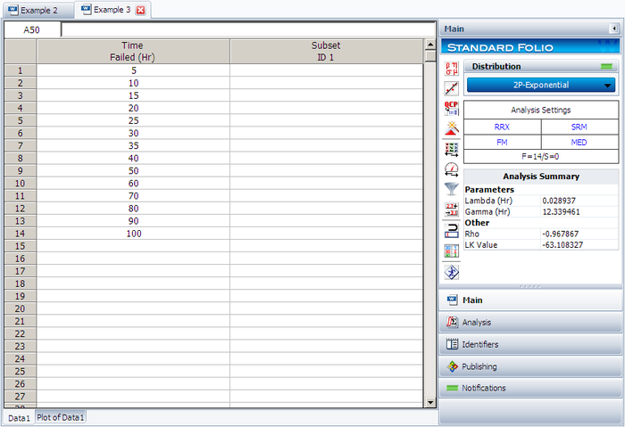
This example can be repeated using Weibull++, choosing 2-parameter exponential and rank regression on Y (RRY), as shown next.

The estimated parameters and the correlation coefficient using Weibull++ were found to be:

[math]\displaystyle{ \hat{\lambda }=0.0271\text{ fr/hr },\hat{\gamma }=10.1348\text{ hr },\hat{\rho }=-0.9679\,\! }[/math]

Please note that the user must deselect the Reset if location parameter > T1 on Exponential option on the Calculations page of the Application Setup window.

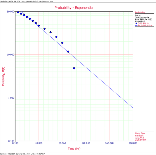
The probability plot can be obtained simply by clicking the Plot icon.

Rank Regression on X

Similar to rank regression on Y, performing a rank regression on X requires that a straight line be fitted to a set of data points such that the sum of the squares of the horizontal deviations from the points to the line is minimized.

Again the first task is to bring our exponential cdf function into a linear form. This step is exactly the same as in regression on Y analysis. The deviation from the previous analysis begins on the least squares fit step, since in this case we treat [math]\displaystyle{ x\,\! }[/math] as the dependent variable and [math]\displaystyle{ y\,\! }[/math] as the independent variable. The best-fitting straight line to the data, for regression on X (see Parameter Estimation), is the straight line:

[math]\displaystyle{ x=\hat{a}+\hat{b}y\,\! }[/math]

The corresponding equations for [math]\displaystyle{ \hat{a}\,\! }[/math] and [math]\displaystyle{ \hat{b}\,\! }[/math] are:

[math]\displaystyle{ \hat{a}=\overline{x}-\hat{b}\overline{y}=\frac{\underset{i=1}{\overset{N}{\mathop{\sum }}}\,{{x}_{i}}}{N}-\hat{b}\frac{\underset{i=1}{\overset{N}{\mathop{\sum }}}\,{{y}_{i}}}{N}\,\! }[/math]

and:

[math]\displaystyle{ \hat{b}=\frac{\underset{i=1}{\overset{N}{\mathop{\sum }}}\,{{x}_{i}}{{y}_{i}}-\tfrac{\underset{i=1}{\overset{N}{\mathop{\sum }}}\,{{x}_{i}}\underset{i=1}{\overset{N}{\mathop{\sum }}}\,{{y}_{i}}}{N}}{\underset{i=1}{\overset{N}{\mathop{\sum }}}\,y_{i}^{2}-\tfrac{{{\left( \underset{i=1}{\overset{N}{\mathop{\sum }}}\,{{y}_{i}} \right)}^{2}}}{N}}\,\! }[/math]

where:

[math]\displaystyle{ \begin{align} {{y}_{i}}=\ln [1-F({{t}_{i}})] \end{align}\,\! }[/math]

and:

[math]\displaystyle{ \begin{align} {{x}_{i}}={{t}_{i}} \end{align}\,\! }[/math]

The values of [math]\displaystyle{ F({{t}_{i}})\,\! }[/math] are estimated from the median ranks. Once [math]\displaystyle{ \hat{a}\,\! }[/math] and [math]\displaystyle{ \hat{b}\,\! }[/math] are obtained, solve for the unknown [math]\displaystyle{ y\,\! }[/math] value, which corresponds to:

[math]\displaystyle{ y=-\frac{\hat{a}}{\hat{b}}+\frac{1}{\hat{b}}x\,\! }[/math]

Solving for the parameters from above equations we get:

[math]\displaystyle{ a=-\frac{\hat{a}}{\hat{b}}=\lambda \gamma \Rightarrow \gamma =\hat{a}\,\! }[/math]

and:

[math]\displaystyle{ b=\frac{1}{\hat{b}}=-\lambda \Rightarrow \lambda =-\frac{1}{\hat{b}}\,\! }[/math]

For the one-parameter exponential case, equations for estimating a and b become:

[math]\displaystyle{ \begin{align} \hat{a}= & 0 \\ \hat{b}= & \frac{\underset{i=1}{\overset{N}{\mathop{\sum }}}\,{{x}_{i}}{{y}_{i}}}{\underset{i=1}{\overset{N}{\mathop{\sum }}}\,y_{i}^{2}} \end{align}\,\! }[/math]

The correlation coefficient is evaluated as before.

RRX Example

2-Parameter Exponential RRX Example

Using the same data set from the RRY example above and assuming a 2-parameter exponential distribution, estimate the parameters and determine the correlation coefficient estimate, [math]\displaystyle{ \hat{\rho }\,\! }[/math], using rank regression on X.

Solution

The table constructed for the RRY analysis applies to this example also. Using the values from this table, we get:

[math]\displaystyle{ \begin{align} \hat{b}= & \frac{\underset{i=1}{\overset{14}{\mathop{\sum }}}\,{{t}_{i}}{{y}_{i}}-\tfrac{\underset{i=1}{\overset{14}{\mathop{\sum }}}\,{{t}_{i}}\underset{i=1}{\overset{14}{\mathop{\sum }}}\,{{y}_{i}}}{14}}{\underset{i=1}{\overset{14}{\mathop{\sum }}}\,y_{i}^{2}-\tfrac{{{\left( \underset{i=1}{\overset{14}{\mathop{\sum }}}\,{{y}_{i}} \right)}^{2}}}{14}} \\ \\ \hat{b}= & \frac{-927.4899-(630)(-13.2315)/14}{22.1148-{{(-13.2315)}^{2}}/14} \end{align}\,\! }[/math]

or:

[math]\displaystyle{ \hat{b}=-34.5563\,\! }[/math]

and:

[math]\displaystyle{ \hat{a}=\overline{x}-\hat{b}\overline{y}=\frac{\underset{i=1}{\overset{14}{\mathop{\sum }}}\,{{t}_{i}}}{14}-\hat{b}\frac{\underset{i=1}{\overset{14}{\mathop{\sum }}}\,{{y}_{i}}}{14}\,\! }[/math]

or:

[math]\displaystyle{ \hat{a}=\frac{630}{14}-(-34.5563)\frac{(-13.2315)}{14}=12.3406\,\! }[/math]

Therefore:

[math]\displaystyle{ \hat{\lambda }=-\frac{1}{\hat{b}}=-\frac{1}{(-34.5563)}=0.0289\text{ failures/hour}\,\! }[/math]

and:

[math]\displaystyle{ \hat{\gamma }=\hat{a}=12.3406\,\! }[/math]

The correlation coefficient is found to be:

[math]\displaystyle{ \hat{\rho }=-0.9679\,\! }[/math]

Note that the equation for regression on Y is not necessarily the same as that for the regression on X. The only time when the two regression methods yield identical results is when the data lie perfectly on a line. If this were the case, the correlation coefficient would be [math]\displaystyle{ -1\,\! }[/math]. The negative value of the correlation coefficient is due to the fact that the slope of the exponential probability plot is negative.

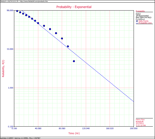
This example can be repeated using Weibull++, choosing two-parameter exponential and rank regression on X (RRX) methods for analysis, as shown below. The estimated parameters and the correlation coefficient using Weibull++ were found to be:

[math]\displaystyle{ \begin{array}{*{35}{l}} \hat{\lambda }= &0.0289 \text{failures/hour} \\ \hat{\gamma}= & 12.3395 \text{hours} \\ \hat{\rho} = &-0.9679 \\ \end{array}\,\! }[/math]

The probability plot can be obtained simply by clicking the Plot icon.

Maximum Likelihood Estimation

As outlined in Parameter Estimation, maximum likelihood estimation works by developing a likelihood function based on the available data and finding the values of the parameter estimates that maximize the likelihood function. This can be achieved by using iterative methods to determine the parameter estimate values that maximize the likelihood function. This can be rather difficult and time-consuming, particularly when dealing with the three-parameter distribution. Another method of finding the parameter estimates involves taking the partial derivatives of the likelihood equation with respect to the parameters, setting the resulting equations equal to zero, and solving simultaneously to determine the values of the parameter estimates. The log-likelihood functions and associated partial derivatives used to determine maximum likelihood estimates for the exponential distribution are covered in Appendix D.

MLE Example

MLE for the Exponential Distribution

Using the same data set from the RRY and RRX examples above and assuming a 2-parameter exponential distribution, estimate the parameters using the MLE method.

Solution

In this example, we have complete data only. The partial derivative of the log-likelihood function, [math]\displaystyle{ \Lambda ,\,\! }[/math] is given by:

[math]\displaystyle{ \frac{\partial \Lambda }{\partial \lambda }=\underset{i=1}{\overset{{{F}_{e}}}{\mathop \sum }}\,\left[ \frac{1}{\lambda }-\left( {{T}_{i}}-\gamma \right) \right]=\underset{i=1}{\overset{14}{\mathop \sum }}\,\left[ \frac{1}{\lambda }-\left( {{T}_{i}}-\gamma \right) \right]=0\,\! }[/math]

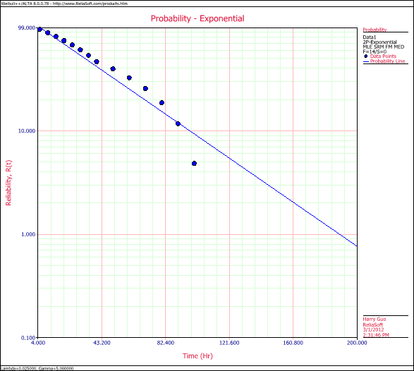
Complete descriptions of the partial derivatives can be found in Appendix D. Recall that when using the MLE method for the exponential distribution, the value of [math]\displaystyle{ \gamma \,\! }[/math] is equal to that of the first failure time. The first failure occurred at 5 hours, thus [math]\displaystyle{ \gamma =5\,\! }[/math] hours[math]\displaystyle{ .\,\! }[/math] Substituting the values for [math]\displaystyle{ T\,\! }[/math] and [math]\displaystyle{ \gamma \,\! }[/math] we get:

[math]\displaystyle{ \frac{14}{\hat{\lambda }}=560\,\! }[/math]

or:

[math]\displaystyle{ \hat{\lambda }=0.025\text{ failures/hour}\,\! }[/math]

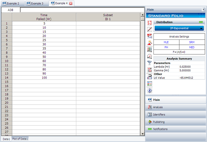
Using Weibull++:

The probability plot is: