Response Surface Methods for Optimization

The experiment designs mentioned in Two Level Factorial Experiments and Highly Fractional Factorial Designs help the experimenter identify factors that affect the response. Once the important factors have been identified, the next step is to determine the settings for these factors that result in the optimum value of the response. The optimum value of the response may either be a maximum value or a minimum value, depending upon the product or process in question. For example, if the response in an experiment is the yield from a chemical process, then the objective might be to find the settings of the factors affecting the yield so that the yield is maximized. On the other hand, if the response in an experiment is the number of defects, then the goal would be to find the factor settings that minimize the number of defects. Methodologies that help the experimenter reach the goal of optimum response are referred to as response surface methods. These methods are exclusively used to examine the "surface," or the relationship between the response and the factors affecting the response. Regression models are used for the analysis of the response, as the focus now is on the nature of the relationship between the response and the factors, rather than identification of the important factors.

Response surface methods usually involve the following steps:

1. The experimenter needs to move from the present operating conditions to the vicinity of the operating conditions where the response is optimum. This is done using the method of steepest ascent in the case of maximizing the response. The same method can be used to minimize the response and is then referred to as the method of steepest descent.
2. Once in the vicinity of the optimum response the experimenter needs to fit a more elaborate model between the response and the factors. Special experiment designs, referred to as RSM designs, are used to accomplish this. The fitted model is used to arrive at the best operating conditions that result in either a maximum or minimum response.
3. It is possible that a number of responses may have to be optimized at the same time. For example, an experimenter may want to maximize strength, while keeping the number of defects to a minimum. The optimum settings for each of the responses in such cases may lead to conflicting settings for the factors. A balanced setting has to be found that gives the most appropriate values for all the responses. Desirability functions are useful in these cases.

Method of Steepest Ascent

The first step in obtaining the optimum response settings, after the important factors have been identified, is to explore the region around the current operating conditions to decide what direction needs to be taken to move towards the optimum region. Usually, a first order regression model (containing just the main effects and no interaction terms) is sufficient at the current operating conditions because the operating conditions are normally far from the optimum response settings. The experimenter needs to move from the current operating conditions to the optimum region in the most efficient way by using the minimum number of experiments. This is done using the method of steepest ascent. In this method, the contour plot of the first order model is used to decide the settings for the next experiment, in order to move towards the optimum conditions. Consider a process where the response has been found to be a function of two factors. To explore the region around the current operating conditions, the experimenter fits the following first order model between the response and the two factors:

[math]\displaystyle{ y={{\beta }_{0}}+{{\beta }_{1}}{{x}_{1}}+{{\beta }_{2}}{{x}_{2}}+\epsilon \,\! }[/math]

The response surface plot for the model, along with the contours, is shown in the figure below. It can be seen in the figure that in order to maximize the response, the most efficient direction in which to move the experiment is along the line perpendicular to the contours. This line, also referred to as the path of steepest ascent, is the line along which the rate of increase of the response is maximum. The steps along this line to move towards the optimum region are proportional to the regression coefficients, [math]\displaystyle{ {{\beta }_{j}},\,\! }[/math] of the fitted first order model.

Experiments are conducted along each step of the path of steepest ascent until an increase in the response is not seen. Then, a new first order model is fit at the region of the maximum response. If the first order model shows a lack of fit, then this indicates that the experimenter has reached the vicinity of the optimum. RSM designs are then used explore the region thoroughly and obtain the point of the maximum response. If the first order model does not show a lack of fit, then a new path of steepest ascent is determined and the process is repeated.

Example

The yield from a chemical process is found to be affected by two factors: reaction temperature and reaction time. The current reaction temperature is 230 [math]\displaystyle{ F\,\! }[/math] and the reaction time is 65 minutes. The experimenter wants to determine the settings of the two factors such that maximum yield can be obtained from the process. To explore the region around the current operating conditions, the experimenter decides to use a single replicate of the [math]\displaystyle{ 2^{2}\,\! }[/math] design. The range of the factors for this design are chosen to be (225, 235) [math]\displaystyle{ F\,\! }[/math] for the reaction temperature and (55, 75) minutes for the reaction time. The unreplicated [math]\displaystyle{ 2^{2}\,\! }[/math] design is also augmented with five runs at the center point to estimate the error sum of squares, [math]\displaystyle{ S{{S}_{E}}\,\! }[/math], and check for model adequacy. The response values obtained for this design are shown next.

In a DOE folio, this design can be set up using the properties shown next.

The resulting design and the analysis results are shown next.

Note that the results shown are in terms of the coded values of the factors (taking -1 as the value of the lower settings for reaction temperature and reaction time and +1 as the value for the higher settings for these two factors). The results show that the factors, [math]\displaystyle{ A\,\! }[/math] (temperature) and [math]\displaystyle{ B\,\! }[/math] (time), affect the response significantly but their interaction does not affect the response. Therefore the interaction term can be dropped from the model for this experiment. The results also show that Curvature is not a significant factor. This indicates that the first order model is adequate for the experiment at the current operating conditions. Using these two conclusions, the model for the current operating conditions, in terms the coded variables is:

[math]\displaystyle{ \hat{y}=36.6375+1.1635x_{1}+0.4875x_{2}\,\! }[/math]

where [math]\displaystyle{ \hat{y}\,\! }[/math] represents the yield and [math]\displaystyle{ x_{1}\,\! }[/math] and [math]\displaystyle{ x_{2}\,\! }[/math] are the predictor variables for the two factors, [math]\displaystyle{ A\,\! }[/math] and [math]\displaystyle{ B\,\! }[/math], respectively. To further confirm the adequacy of the model of the equation given above, the experiment can be analyzed again after dropping the interaction term, [math]\displaystyle{ AB\,\! }[/math]. The results are shown next.

The results show that the lack-of-fit for this model (because of the deficiency created in the model by the absence of the interaction term) is not significant, confirming that the model is adequate.

Path of Steepest Ascent

The contour plot for the model used in the above example is shown next.

The regression coefficients for the model are [math]\displaystyle{ \hat{\beta}_{1}= 1.1625\,\! }[/math] and [math]\displaystyle{ \hat{\beta}_{2}= 0.4875\,\! }[/math]. To move towards the optimum, the experimenter needs to move along the path of steepest ascent, which lies perpendicular to the contours. This path is the line through the center point of the current operating conditions ([math]\displaystyle{ x_{1}=0\,\! }[/math], [math]\displaystyle{ x_{2}=0\,\! }[/math]) with a slope of [math]\displaystyle{ \hat{\beta}_{2}/\hat{\beta}_{1}\,\! }[/math]. Therefore, in terms of the coded variables, the experiment should be moved 1.1625 units in the [math]\displaystyle{ x_{1}\,\! }[/math] direction for every 0.4875 units in the [math]\displaystyle{ x_{2}\,\! }[/math] direction. To move along this path, the experimenter decides to use a step-size of 10 minutes for the reaction time, [math]\displaystyle{ x_{2}\,\! }[/math]. The coded value for this step size can be obtained as follows. Recall from Multiple Linear Regression Analysis that the relationship between coded and actual values is:

[math]\displaystyle{ coded\ value=\frac{actual\ value - mean}{half\ of\ range} }[/math]

or

[math]\displaystyle{ coded\ value=\frac{step\ size\ in\ actual\ value}{half\ of\ range} }[/math]

Thus, for a step-size of 10 minutes, the equivalent step size in coded value for [math]\displaystyle{ x_{2}\,\! }[/math] is:

[math]\displaystyle{ =\frac{10}{half\ of\ range\ of\ x_{2}}\,\! }[/math]

[math]\displaystyle{ =\frac{10}{(75-55)/2}\,\! }[/math]

[math]\displaystyle{ =1\,\! }[/math]

In terms of the coded variables, the path of steepest ascent requires a move of 1.1625 units in the [math]\displaystyle{ x_{1}\,\! }[/math] direction for every 0.4875 units in the [math]\displaystyle{ x_{2}\,\! }[/math] direction. The step-size for [math]\displaystyle{ x_{1}\,\! }[/math], in terms of the coded value corresponding to any step-size in [math]\displaystyle{ x_{2}\,\! }[/math], is:

[math]\displaystyle{ =\frac{\hat{\beta_{1}}}{\hat{\beta_{2}}}\cdot(step\ size\ in\ x_{2})\,\! }[/math]

Therefore, the step-size for the reaction temperature, [math]\displaystyle{ x_{1}\,\! }[/math], in terms of the coded variables is:

[math]\displaystyle{ =\frac{\hat{\beta_{1}}}{\hat{\beta_{2}}}\cdot\Delta x_{2}\,\! }[/math]

[math]\displaystyle{ =\frac{1.1625}{0.4875}\cdot1\,\! }[/math]

[math]\displaystyle{ =\frac{\hat{\beta_{1}}}{\hat{\beta_{2}}}\cdot\Delta x_{2}\,\! }[/math]

This corresponds to a step of approximately 12 [math]\displaystyle{ F\,\! }[/math] for temperature in terms of the actual value as shown next:

[math]\displaystyle{ \begin{align} step\ size\ in\ actual\ value = & (coded\ value)\cdot(half\ of\ the\ range\ of\ x_{1})\\ = & 2.39\cdot10/2\\ = & 11.95 \end{align}\,\! }[/math]

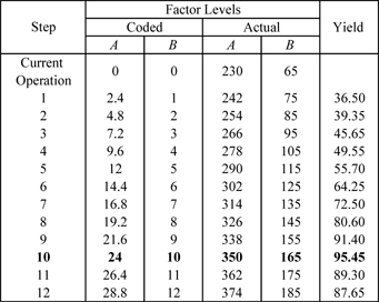
Using a step of 12 [math]\displaystyle{ F\,\! }[/math] and 10 minutes, the experimenter conducts experiments until no further increase is observed in the yield. The yield values at each step are shown in the table given next.

The yield starts decreasing after the reaction temperature of 350 [math]\displaystyle{ F\,\! }[/math] and the reaction time of 165 minutes, indicating that this point may lie close to the optimum region. To analyze the vicinity of this point, a [math]\displaystyle{ 2^{2}\,\! }[/math] design augmented by five center points is selected. The range of exploration is chosen to be 345 to 355 [math]\displaystyle{ F\,\! }[/math] for reaction temperature and 155 to 175 minutes for reaction time. The response values recorded are shown next.

The results for this design are shown next.

In the results, Curvature is displayed as a significant factor. This indicates that the first order model is not adequate for this region of the experiment and a higher order model is required. As a result, the methodology of steepest ascent can no longer be used. The presence of curvature indicates that the experiment region may be close to the optimum. Special designs that allow the use of second order models are needed at this point.

RSM Designs

A second order model is generally used to approximate the response once it is realized that the experiment is close to the optimum response region where a first order model is no longer adequate. The second order model is usually sufficient for the optimum region, as third order and higher effects are seldom important. The second order regression model takes the following form for [math]\displaystyle{ k\,\! }[/math] factors:

[math]\displaystyle{ \begin{align} y= & {{\beta }_{0}}+{{\beta }_{1}}{{x}_{1}}+{{\beta }_{2}}{{x}_{2}}+...+{{\beta }_{k}}{{x}_{k}}+ \\ & {{\beta }_{11}}x_{1}^{2}+{{\beta }_{22}}x_{2}^{2}+...+{{\beta }_{kk}}x_{k}^{2}+{{\beta }_{12}}{{x}_{1}}{{x}_{2}}+...+{{\beta }_{k-1,k}}{{x}_{k-1}}{{x}_{k}}+\epsilon \end{align}\,\! }[/math]

The model contains [math]\displaystyle{ p=(k+1)(k+2)/2\,\! }[/math] regression parameters that include coefficients for main effects ([math]\displaystyle{ {{\beta }_{1}},{{\beta }_{2}}...{{\beta }_{k}}\,\! }[/math]), coefficients for quadratic main effects ([math]\displaystyle{ {{\beta }_{11}},{{\beta }_{22}}...{{\beta }_{kk}}\,\! }[/math]) and coefficients for two factor interaction effects ([math]\displaystyle{ {{\beta }_{12}},{{\beta }_{13}}\,\! }[/math]... [math]\displaystyle{ {{\beta }_{k-1,k}}\,\! }[/math]). A full factorial design with all factors at three levels would provide estimation of all the required regression parameters. However, full factorial three level designs are expensive to use as the number of runs increases rapidly with the number of factors. For example, a three factor full factorial design with each factor at three levels would require [math]\displaystyle{ {{3}^{3}}=27\,\! }[/math] runs while a design with four factors would require [math]\displaystyle{ {{3}^{4}}=81\,\! }[/math] runs. Additionally, these designs will estimate a number of higher order effects which are usually not of much importance to the experimenter. Therefore, for the purpose of analysis of response surfaces, special designs are used that help the experimenter fit the second order model to the response with the use of a minimum number of runs. Examples of these designs are the central composite and Box-Behnken designs.

Central Composite Designs

Central composite designs are two level full factorial ([math]\displaystyle{ 2^{k}\,\! }[/math]) or fractional factorial ([math]\displaystyle{ 2^{k-f}\,\! }[/math]) designs augmented by a number of center points and other chosen runs. These designs are such that they allow the estimation of all the regression parameters required to fit a second order model to a given response.

The simplest of the central composite designs can be used to fit a second order model to a response with two factors. The design consists of a [math]\displaystyle{ 2^{2}\,\! }[/math] full factorial design augmented by a few runs at the center point (such a design is shown in figure (a) given below). A central composite design is obtained when runs at points ([math]\displaystyle{ -1,0\,\! }[/math]), ([math]\displaystyle{ 1,0\,\! }[/math]), ([math]\displaystyle{ 0,-1\,\! }[/math]) and ([math]\displaystyle{ 0,1\,\! }[/math]) are added to this design. These points are referred to as axial points or star points and represent runs where all but one of the factors are set at their mid-levels. The number of axial points in a central composite design having [math]\displaystyle{ k\,\! }[/math] factors is [math]\displaystyle{ 2k\,\! }[/math]. The distance of the axial points from the center point is denoted by [math]\displaystyle{ \alpha \,\! }[/math] and is always specified in terms of coded values. For example, the central composite design in figure (b) given below has [math]\displaystyle{ \alpha =1\,\! }[/math], while for the design of figure (c) [math]\displaystyle{ \alpha =1.414\,\! }[/math].

It can be noted that when [math]\displaystyle{ \alpha \gt 1\,\! }[/math], each factor is run at five levels ([math]\displaystyle{ -\alpha \,\! }[/math], [math]\displaystyle{ -1\,\! }[/math], [math]\displaystyle{ 0\,\! }[/math], [math]\displaystyle{ 1\,\! }[/math] and [math]\displaystyle{ \alpha \,\! }[/math]) instead of the three levels of [math]\displaystyle{ -1\,\! }[/math], [math]\displaystyle{ 0\,\! }[/math] and [math]\displaystyle{ 1\,\! }[/math]. The reason for running central composite designs with [math]\displaystyle{ \alpha \gt 1\,\! }[/math] is to have a rotatable design, which is explained next.

Rotatability

A central composite design is said to be rotatable if the variance of any predicted value of the response, [math]\displaystyle{ {{\hat{y}}_{p}}\,\! }[/math], for any level of the factors depends only on the distance of the point from the center of the design, regardless of the direction. In other words, a rotatable central composite design provides constant variance of the estimated response corresponding to all new observation points that are at the same distance from the center point of the design (in terms of the coded variables).

The variance of the predicted response at any point, [math]\displaystyle{ {{x}_{p}}\,\! }[/math], is given as follows:

[math]\displaystyle{ V[{{\hat{y}}_{p}}]={{\sigma }^{2}}x_{p}^{\prime }{{({{X}^{\prime }}X)}^{-1}}{{x}_{p}}\,\! }[/math]

The contours of [math]\displaystyle{ V[{{\hat{y}}_{p}}]\,\! }[/math] for the central composite design in figure (c) above are shown in the figure below. The contours are concentric circles indicating that the central composite design of figure (c) is rotatable. Rotatability is a desirable property because the experimenter does not have any prior information about the location of the optimum. Therefore, a design that provides equal precision of estimation in all directions would be preferred. Such a design will assure the experimenter that no matter what direction is taken to search for the optimum, he/she will be able to estimate the response value with equal precision. A central composite design is rotatable if the value of [math]\displaystyle{ \alpha \,\! }[/math] for the design satisfies the following equation:

[math]\displaystyle{ \alpha ={{\left[ \frac{{{2}^{k-f}}({{n}_{f}})}{{{n}_{s}}} \right]}^{1/4}}\,\! }[/math]

where [math]\displaystyle{ {{n}_{f}}\,\! }[/math] is the number of replicates of the runs in the original factorial design and [math]\displaystyle{ {{n}_{s}}\,\! }[/math] is the number of replicates of the runs at the axial points. For example, a central composite design with two factors, having a single replicate of the original factorial design, and a single replicate of all the axial points, would be rotatable for the following [math]\displaystyle{ \alpha \,\! }[/math] value:

[math]\displaystyle{ \begin{align} \alpha = & {{\left[ \frac{{{2}^{k-f}}({{n}_{f}})}{{{n}_{s}}} \right]}^{1/4}} \\ = & {{\left[ \frac{{{2}^{2}}(1)}{1} \right]}^{1/4}} \\ = & \sqrt{2} \\ = & 1.414 \end{align}\,\! }[/math]

Thus, a central composite design in two factors, having a single replicate of the original [math]\displaystyle{ 2^{2}\,\! }[/math] design and axial points, and with [math]\displaystyle{ \alpha =1.414\,\! }[/math], is a rotatable design. This design is shown in figure (c) above.

Spherical Design

A central composite design is said to be spherical if all factorial and axial points are at same distance from the center of the design. Spherical central composite designs are obtained by setting [math]\displaystyle{ \alpha =\sqrt{k}\,\! }[/math]. For example, the rotatable design in the figure above (c) is also a spherical design because for this design [math]\displaystyle{ \alpha =\sqrt{k}=\sqrt{2}=1.414\,\! }[/math].

Face-centered Design

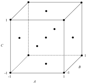
Central composite designs in which the axial points represent the mid levels for all but one of the factors are also referred to as face-centered central composite designs. For these designs, [math]\displaystyle{ \alpha =1\,\! }[/math] and all factors are run at three levels, which are [math]\displaystyle{ -1\,\! }[/math], [math]\displaystyle{ 0\,\! }[/math] and [math]\displaystyle{ 1,\,\! }[/math] in terms of the coded values (see the figure below).

Box-Behnken Designs

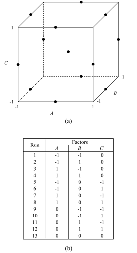
In Highly Fractional Factorial Designs, highly fractional designs introduced by Plackett and Burman were discussed. Plackett-Burman designs are used to estimate main effects in the case of two level fractional factorial experiments using very few runs. [G. E. P. Box and D. W. Behnken (1960)] introduced similar designs for three level factors that are widely used in response surface methods to fit second-order models to the response. The designs are referred to as Box-Behnken designs. The designs were developed by the combination of two level factorial designs with incomplete block designs. For example, the figure below shows the Box-Behnken design for three factors. The design is obtained by the combination of [math]\displaystyle{ 2^{2}\,\! }[/math] design with a balanced incomplete block design having three treatments and three blocks (for details see [Box 1960, Montgomery 2001]).

The advantages of Box-Behnken designs include the fact that they are all spherical designs and require factors to be run at only three levels. The designs are also rotatable or nearly rotatable. Some of these designs also provide orthogonal blocking. Thus, if there is a need to separate runs into blocks for the Box-Behnken design, then designs are available that allow blocks to be used in such a way that the estimation of the regression parameters for the factor effects are not affected by the blocks. In other words, in these designs the block effects are orthogonal to the other factor effects. Yet another advantage of these designs is that there are no runs where all factors are at either the [math]\displaystyle{ +1\,\! }[/math] or [math]\displaystyle{ -1\,\! }[/math] levels. For example, in the figure below the representation of the Box-Behnken design for three factors clearly shows that there are no runs at the corner points. This could be advantageous when the corner points represent runs that are expensive or inconvenient because they lie at the end of the range of the factor levels. A few of the Box-Behnken designs available in DOE++ are presented in Appendix F.

Example

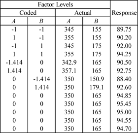
Continuing with the example in Method of Steepest Ascent, the first order model was found to be inadequate for the region near the optimum. Once the experimenter realized that the first order model was not adequate (for the region with a reaction temperature of 350 [math]\displaystyle{ F\,\! }[/math] and reaction time of 165 minutes), it was decided to augment the experiment with axial runs to be able to complete a central composite design and fit a second order model to the response. Notice the advantage of using a central composite design, as the experimenter only had to add the axial runs to the [math]\displaystyle{ 2^{2}\,\! }[/math] design with center point runs, and did not have to begin a new experiment. The experimenter decided to use [math]\displaystyle{ \alpha =1.4142\,\! }[/math] to get a rotatable design. The obtained response values are shown in the figure below.

Such a design can be set up in a Weibull++ DOE folio using the properties shown in the figure below.

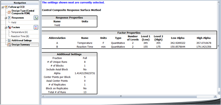
The resulting design is shown in the figure shown next.

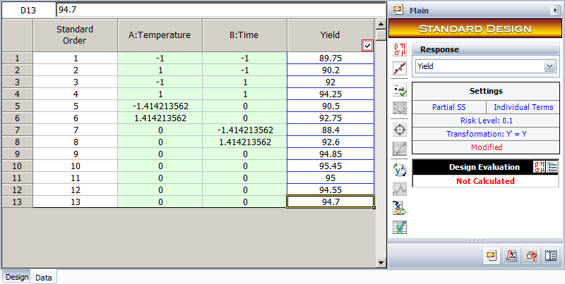
Results from the analysis of the design are shown in the next figure.

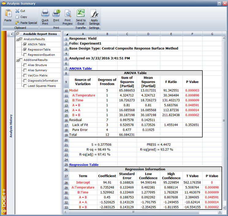
The results in the figure above show that the main effects, [math]\displaystyle{ A\,\! }[/math] and [math]\displaystyle{ B\,\! }[/math], the interaction, [math]\displaystyle{ AB\,\! }[/math], and the quadratic main effects, [math]\displaystyle{ {{A}^{2}}\,\! }[/math] and [math]\displaystyle{ {{B}^{2}}\,\! }[/math], (represented as AA and BB in the figure) are significant. The lack-of-fit test also shows that the second order model with these terms is adequate and a higher order model is not needed. Using these results, the model for the experiment in terms of the coded values is:

[math]\displaystyle{ \hat{y}=94.91+0.74{{x}_{1}}+1.53{{x}_{2}}+0.45{{x}_{1}}{{x}_{2}}-1.52x_{1}^{2}-2.08x_{2}^{2}\,\! }[/math]

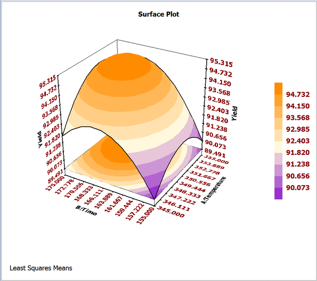
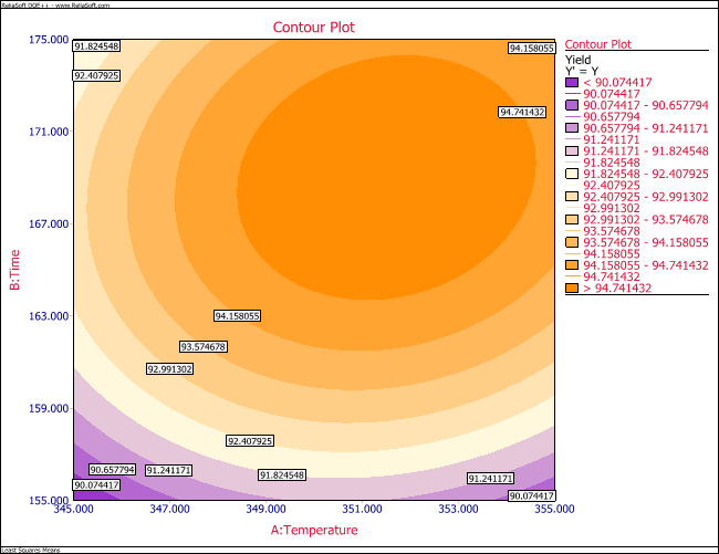
The response surface and the contour plot for this model, in terms of the actual variables, are shown in the below figures (a) and (b), respectively.

Analysis of the Second Order Model

Once a second order model is fit to the response, the next step is to locate the point of maximum or minimum response. The second order model for [math]\displaystyle{ k\,\! }[/math] factors can be written as:

[math]\displaystyle{ \hat{y}={{\hat{\beta }}_{0}}+\underset{i=1}{\overset{k}{\mathop{\sum }}}\,{{\hat{\beta }}_{i}}{{x}_{i}}+\underset{i=1}{\overset{k}{\mathop{\sum }}}\,{{\hat{\beta }}_{ii}}x_{i}^{2}+\underset{i=1}{\overset{k}{\mathop{\sum }}}\,\underset{j=1}{\overset{i-1}{\mathop{\sum }}}\,{{\hat{\beta }}_{ij}}{{x}_{i}}{{x}_{j}}\,\! }[/math]

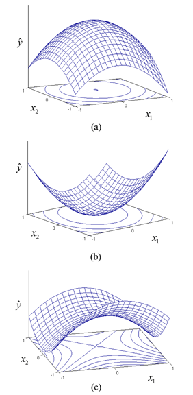
The point for which the response, [math]\displaystyle{ \hat{y}\,\! }[/math], is optimized is the point at which the partial derivatives, [math]\displaystyle{ \partial \hat{y}/\partial {{x}_{1}}\,\! }[/math], [math]\displaystyle{ \partial \hat{y}/\partial {{x}_{2}}\,\! }[/math], [math]\displaystyle{ ...\partial \hat{y}/\partial {{x}_{k}},\,\! }[/math] are all equal to zero. This point is called the stationary point. The stationary point may be a point of maximum response, minimum response or a saddle point. These three conditions are shown in the following figures (a), (b) and (c) respectively.

Notice that these conditions are easy to identify, in the case of two factor experiments, by the inspection of the contour plots. However, when more than two factors exist in an experiment, then the general mathematical solution for the location of the stationary point has to be used. The equation given above can be written in matrix notation as:

[math]\displaystyle{ \hat{y}={{\hat{\beta }}_{0}}+{{x}^{\prime }}b+{{x}^{\prime }}Bx\,\! }[/math]

where:

[math]\displaystyle{ x=\left[ \begin{matrix} {{x}_{1}} \\ {{x}_{2}} \\ . \\ . \\ . \\ {{x}_{k}} \\ \end{matrix} \right]\text{ }b=\left[ \begin{matrix} {{{\hat{\beta }}}_{1}} \\ {{{\hat{\beta }}}_{2}} \\ . \\ . \\ . \\ {{{\hat{\beta }}}_{k}} \\ \end{matrix} \right]\text{ and }B=\left[ \begin{matrix} {{{\hat{\beta }}}_{11}} & {{{\hat{\beta }}}_{12}}/2 & . & . & . & {{{\hat{\beta }}}_{1k}}/2 \\ {} & {{{\hat{\beta }}}_{22}} & . & . & . & {{{\hat{\beta }}}_{2k}}/2 \\ {} & {} & . & . & . & . \\ {} & {} & {} & . & . & . \\ {} & {} & {} & {} & . & . \\ \text{sym}\text{.} & {} & {} & {} & {} & {{{\hat{\beta }}}_{kk}} \\ \end{matrix} \right]\,\! }[/math]

Then the stationary point can be determined as follows:

[math]\displaystyle{ \frac{\partial \hat{y}}{\partial x}=b+2Bx=0\,\! }[/math]

Thus, the stationary point is:

[math]\displaystyle{ {{x}_{s}}=-\frac{1}{2}{{B}^{-1}}b\,\! }[/math]

The optimum response is the response corresponding to [math]\displaystyle{ {{x}_{s}}\,\! }[/math]. The optimum response can be obtained to get:

[math]\displaystyle{ {{\hat{y}}_{s}}={{\hat{\beta }}_{0}}+\frac{1}{2}x_{s}^{\prime }b\,\! }[/math]

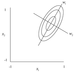
Once the stationary point is known, it is necessary to determine if it is a maximum or minimum or saddle point. To do this, the second order model has to be transformed to the canonical form. This is done by transforming the model to a new coordinate system such that the origin lies at the stationary point and the axes are parallel to the principal axes of the fitted response surface, shown next.

The resulting model equation then takes the following form:

[math]\displaystyle{ \hat{y}={{\hat{y}}_{s}}+{{\lambda }_{1}}w_{1}^{2}+{{\lambda }_{2}}w_{2}^{2}+...+{{\lambda }_{k}}w_{k}^{2}\,\! }[/math]

where the [math]\displaystyle{ {{w}_{i}}\,\! }[/math] s are the transformed independent variables, and [math]\displaystyle{ {{\lambda }_{i}}\,\! }[/math]s are constants that are also the eigenvalues of the matrix [math]\displaystyle{ B\,\! }[/math]. The nature of the stationary point is known by looking at the signs of the [math]\displaystyle{ {{\lambda }_{i}}\,\! }[/math]s. If the [math]\displaystyle{ {{\lambda }_{i}}\,\! }[/math] s are all negative, then [math]\displaystyle{ {{x}_{s}}\,\! }[/math] is a point of maximum response. If the [math]\displaystyle{ {{\lambda }_{i}}\,\! }[/math]s are all positive then [math]\displaystyle{ {{x}_{s}}\,\! }[/math] is a point of minimum response. If the [math]\displaystyle{ {{\lambda }_{i}}\,\! }[/math]s have different signs, then [math]\displaystyle{ {{x}_{s}}\,\! }[/math] is a saddle point.

Example

Continuing with the example in Method of Steepest Ascent, the second order model fitted to the response, in terms of the coded variables, was obtained as:

[math]\displaystyle{ \hat{y}=94.91+0.74{{x}_{1}}+1.53{{x}_{2}}+0.45{{x}_{1}}{{x}_{2}}-1.52x_{1}^{2}-2.08x_{2}^{2}\,\! }[/math]

Then the [math]\displaystyle{ b\,\! }[/math] and [math]\displaystyle{ B\,\! }[/math] matrices for this model are:

[math]\displaystyle{ b=\left[ \begin{matrix} 0.74 \\ 1.53 \\ \end{matrix} \right]\text{ }B=\left[ \begin{matrix} -1.52 & 0.45 \\ 0.45 & -2.08 \\ \end{matrix} \right]\,\! }[/math]

The stationary point is:

[math]\displaystyle{ \begin{align} {{x}_{s}}= & -\frac{1}{2}{{B}^{-1}}b \\ = & -\frac{1}{2}{{\left[ \begin{matrix} -1.52 & 0.45 \\ 0.45 & -2.08 \\ \end{matrix} \right]}^{-1}}\left[ \begin{matrix} 0.74 \\ 1.53 \\ \end{matrix} \right] \\ = & \left[ \begin{matrix} 0.3 \\ 0.4 \\ \end{matrix} \right] \end{align}\,\! }[/math]

Then, in terms of the actual values, the stationary point can be found as:

[math]\displaystyle{ \begin{align} \text{Reaction Temperature:} & 0.3=\frac{T-350}{(355-345)/2} \\ T= & 351.5\text{ }F \end{align}\,\! }[/math]

[math]\displaystyle{ \begin{align} \text{Reaction Time:} & 0.4=\frac{t-165}{(175-155)/2} \\ t= & 169.0\text{ minutes} \end{align}\,\! }[/math]

To find the nature of the stationary point the eigenvalues of the [math]\displaystyle{ B\,\! }[/math] matrix can be obtained as follows using the determinant of the matrix [math]\displaystyle{ B-\lambda I\,\! }[/math]:

[math]\displaystyle{ \begin{align} \left| B-\lambda I \right|= & 0 \\ \left| \begin{matrix} -1.52-\lambda & 0.45 \\ 0.45 & -2.08-\lambda \\ \end{matrix} \right|= & 0 \end{align}\,\! }[/math]

This gives us:

[math]\displaystyle{ {{\lambda }^{2}}+3.61\lambda +2.9743=0\,\! }[/math]

Solving the quadratic equation in [math]\displaystyle{ \lambda \,\! }[/math] returns the eigenvalues [math]\displaystyle{ {{\lambda }_{1}}=-1.2723\,\! }[/math] and [math]\displaystyle{ {{\lambda }_{2}}=-2.3377\,\! }[/math]. Since both the eigenvalues are negative, it can be concluded that the stationary point is a point of maximum response. The predicted value of the maximum response can be obtained as:

[math]\displaystyle{ \begin{align} {{{\hat{y}}}_{s}}= & {{{\hat{\beta }}}_{0}}+\frac{1}{2}x_{s}^{\prime }b \\ = & 94.91+\frac{1}{2}{{\left[ \begin{matrix} 0.3 \\ 0.4 \\ \end{matrix} \right]}^{\prime }}\left[ \begin{matrix} 0.74 \\ 1.53 \\ \end{matrix} \right] \\ = & 95.3 \end{align}\,\! }[/math]

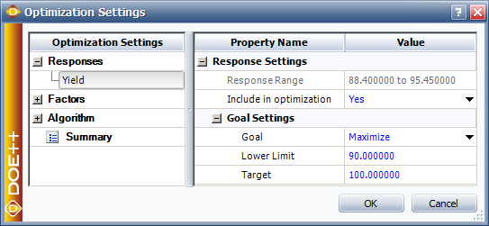
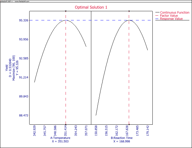
In DOE++, the maximum response can be obtained by entering the required values as shown in the figure below. In the figure, the goal is to maximize the response and the limits of the search range for maximizing the response are entered as 90 and 100. The value of the maximum response and the corresponding values of the factors obtained are shown in the second figure following. These values match the values calculated in this example.

Multiple Responses

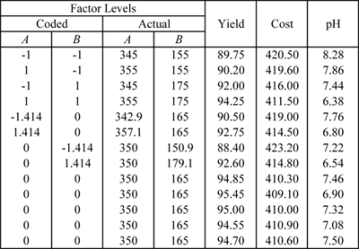
In many cases, the experimenter has to optimize a number of responses at the same time. For the example in Method of Steepest Ascent, assume that the experimenter has to also consider two other responses: cost of the product (which should be minimized) and the pH of the product (which should be close to 7 so that the product is neither acidic nor basic). The data is presented in the figure below.

The problem in dealing with multiple responses is that now there might be conflicting objectives because of the different requirements of each of the responses. The experimenter needs to come up with a solution that satisfies each of the requirements as much as possible without compromising too much on any of the requirements. The approach used in DOE++ to deal with optimization of multiple responses involves the use of desirability functions that are discussed next (for details see [Derringer and Suich, 1980]).

Desirability Functions

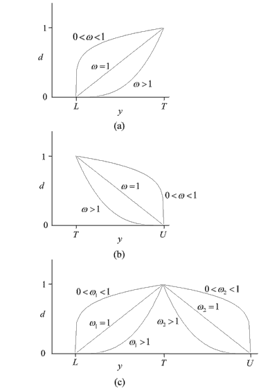
Under this approach, each [math]\displaystyle{ i\,\! }[/math]th response is assigned a desirability function, [math]\displaystyle{ {{d}_{i}}\,\! }[/math], where the value of [math]\displaystyle{ {{d}_{i}}\,\! }[/math] varies between 0 and 1. The function, [math]\displaystyle{ {{d}_{i}},\,\! }[/math] is defined differently based on the objective of the response. If the response is to be maximized, as in the case of the previous example where the yield had to be maximized, then [math]\displaystyle{ {{d}_{i}}\,\! }[/math] is defined as follows:

[math]\displaystyle{ {{d}_{i}}=\left\{ \begin{matrix} 0 & {{y}_{i}}\lt L \\ {{\left( \frac{{{y}_{i}}-L}{T-L} \right)}^{\omega }} & L\le {{y}_{i}}\le T \\ 1 & {{y}_{i}}\gt T \\ \end{matrix} \right. }[/math]

where [math]\displaystyle{ T\,\! }[/math] represents the target value of the [math]\displaystyle{ i\,\! }[/math]th response, [math]\displaystyle{ {{y}_{i}}\,\! }[/math], [math]\displaystyle{ L\,\! }[/math] represents the acceptable lower limit value for this response and [math]\displaystyle{ \omega \,\! }[/math] represents the weight. When [math]\displaystyle{ \omega =1\,\! }[/math] the function [math]\displaystyle{ {{d}_{i}}\,\! }[/math] is linear. If [math]\displaystyle{ \omega \gt 1\,\! }[/math] then more importance is placed on achieving the target for the response, [math]\displaystyle{ {{y}_{i}}\,\! }[/math]. When [math]\displaystyle{ \omega \lt 1\,\! }[/math], less weight is assigned to achieving the target for the response, [math]\displaystyle{ {{y}_{i}}\,\! }[/math]. A graphical representation is shown in figure (a) below.

If the response is to be minimized, as in the case when the response is cost, [math]\displaystyle{ {{d}_{i}}\,\! }[/math] is defined as follows:

[math]\displaystyle{ {{d}_{i}}=\left\{ \begin{matrix} 1 & {{y}_{i}}\lt T \\ {{\left( \frac{U-{{y}_{i}}}{U-T} \right)}^{\omega }} & T\le {{y}_{i}}\le U \\ 0 & {{y}_{i}}\gt U \\ \end{matrix} \right. }[/math]

Here [math]\displaystyle{ U\,\! }[/math] represents the acceptable upper limit for the response (see figure (b) above).

There may be times when the experimenter wants the response to be neither maximized nor minimized, but instead stay as close to a specified target as possible. For example, in the case where the experimenter wants the product to be neither acidic nor basic, there is a requirement to keep the pH close to the neutral value of 7. In such cases, the desirability function is defined as follows (see figure (c) above):

[math]\displaystyle{ {{d}_{i}}=\left\{ \begin{matrix} 0 & {{y}_{i}}\lt L \\ {{\left( \frac{{{y}_{i}}-L}{T-L} \right)}^{{{\omega }_{1}}}} & L\le {{y}_{i}}\le T \\ {{\left( \frac{U-{{y}_{i}}}{U-T} \right)}^{{{\omega }_{2}}}} & T\le {{y}_{i}}\le U \\ 0 & {{y}_{i}}\gt U \\ \end{matrix} \right. }[/math]

Once a desirability function is defined for each of the responses, assuming that there are [math]\displaystyle{ m\,\! }[/math] responses, an overall desirability function is obtained as follows:

[math]\displaystyle{ D={{(d_{1}^{{{r}_{1}}}\cdot d_{2}^{{{r}_{2}}}\cdot ...\cdot d_{m}^{{{r}_{m}}})}^{1/({{r}_{1}}+{{r}_{2}}+...+{{r}_{m}})}}\,\! }[/math]

where the [math]\displaystyle{ {{r}_{i}}\,\! }[/math] s represent the importance of each response. The greater the value of [math]\displaystyle{ {{r}_{i}}\,\! }[/math], the more important the response with respect to the other responses. The objective is to now find the settings that return the maximum value of [math]\displaystyle{ D\,\! }[/math].

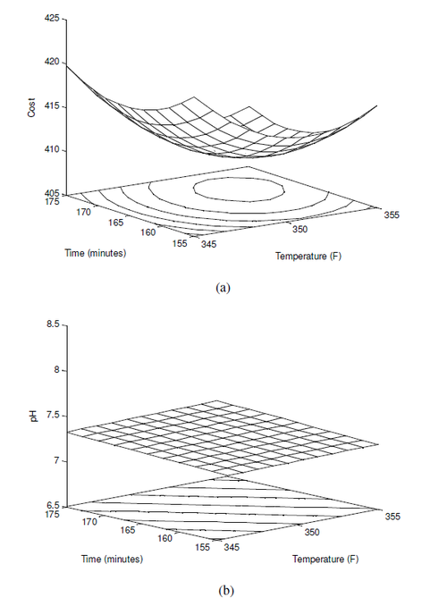
To illustrate the use of desirability functions, consider the previous example with the three responses of yield, cost and pH. The response surfaces for the two additional responses of cost and pH are shown next in the figures (a) and (b), respectively.

In terms of actual variables, the models obtained for all three responses are as shown next:

[math]\displaystyle{ \begin{align} \text{Yield: } & {{{\hat{y}}}_{1}}=-7480.24+41.24{{x}_{1}}+3.88{{x}_{2}}+0.009{{x}_{1}}{{x}_{2}} \\ & -0.060825x_{1}^{2}-0.020831x_{2}^{2} \\ \text{Cost: } & {{{\hat{y}}}_{2}}=15560.49-82.48{{x}_{1}}-7.76{{x}_{2}}-0.02{{x}_{1}}{{x}_{2}} \\ & +0.12165x_{1}^{2}+0.041663x_{2}^{2} \\ \text{pH: } & {{{\hat{y}}}_{3}}=38.87-0.0709{{x}_{1}}-0.041{{x}_{2}} \end{align}\,\! }[/math]

Assume that the experimenter wants to have a target yield value of 95, although any value of yield greater than 94 is acceptable. Then the desirability function for yield is:

[math]\displaystyle{ {{d}_{1}}=\left\{ \begin{matrix} 0 & {{y}_{1}}\lt 94 \\ {{\left( \frac{{{y}_{1}}-94}{95-94} \right)}^{\omega }} & 94\le {{y}_{1}}\le 95 \\ 1 & {{y}_{1}}\gt 95 \\ \end{matrix} \right. }[/math]

For the cost, assume that the experimenter wants to lower the cost to 400, although any cost value below 415 is acceptable. Then the desirability function for cost is:

[math]\displaystyle{ {{d}_{2}}=\left\{ \begin{matrix} 1 & {{y}_{2}}\lt 400 \\ {{\left( \frac{415-{{y}_{2}}}{415-400} \right)}^{\omega }} & 400\le {{y}_{2}}\le 415 \\ 0 & {{y}_{2}}\gt 415 \\ \end{matrix} \right. }[/math]

For the pH, a target of 7 is desired but values between 6.9 and 7.1 are also acceptable. Thus, the desirability function here is:

[math]\displaystyle{ {{d}_{3}}=\left\{ \begin{matrix} 0 & {{y}_{3}}\lt L \\ {{\left( \frac{{{y}_{3}}-6.9}{7-6.9} \right)}^{{{\omega }_{1}}}} & 6.9\le {{y}_{3}}\le 7 \\ {{\left( \frac{7.1-{{y}_{3}}}{7.1-7} \right)}^{{{\omega }_{2}}}} & 7\le {{y}_{3}}\le 7.1 \\ 0 & {{y}_{3}}\gt 7.1 \\ \end{matrix} \right. }[/math]

Notice that in the previous equations all weights used ([math]\displaystyle{ {{\omega }_{i}}\,\! }[/math] s) are 1. Thus, all three desirability functions are linear. The overall desirability function, assuming equal importance ([math]\displaystyle{ {{r}_{1}}={{r}_{2}}={{r}_{3}}=1\,\! }[/math]) for all the responses, is:

[math]\displaystyle{ \begin{align} D= & {{({{d}_{1}}\cdot {{d}_{2}}\cdot {{d}_{3}})}^{1/3}} \\ = & f({{{\hat{y}}}_{1}},{{{\hat{y}}}_{2}},{{{\hat{y}}}_{3}}) \end{align}\,\! }[/math]

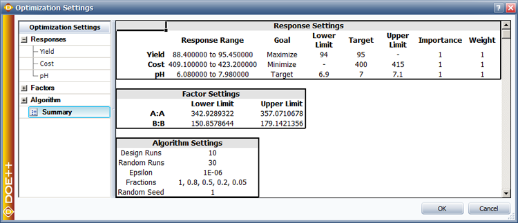
The objective of the experimenter is to find the settings of [math]\displaystyle{ {{x}_{1}}\,\! }[/math] and [math]\displaystyle{ {{x}_{2}}\,\! }[/math] such that the overall desirability, [math]\displaystyle{ D\,\! }[/math], is maximum. In DOE++, the settings for the desirability functions for each of the three responses can be entered as shown in the next figure.

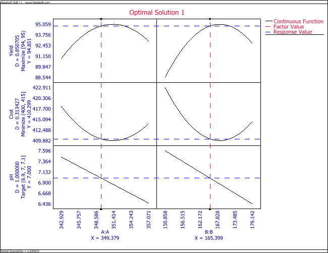
Based on these settings, DOE++ solves this optimization problem to obtain the following solution:

[math]\displaystyle{ \begin{align} Temperature= & 351.5\text{ }F\text{ } \\ Time= & 169\text{ }minutes \end{align}\,\! }[/math]

The overall desirability achieved with this solution can be calculated easily. The values of each of the response for these settings are:

[math]\displaystyle{ \begin{align} \text{ }{{{\hat{y}}}_{1}}= & -7480.24+41.24{{x}_{1}}+3.88{{x}_{2}}+0.009{{x}_{1}}{{x}_{2}} \\ & -0.060825x_{1}^{2}-0.020831x_{2}^{2} \\ = & -7480.24+41.24(351.5)+3.88(169)+0.009(351.3)(169) \\ & -0.060825{{(351.5)}^{2}}-0.020831{{(169)}^{2}} \\ = & 95.3 \\ \text{ }{{{\hat{y}}}_{2}}= & 15560.49-82.48{{x}_{1}}-7.76{{x}_{2}}-0.02{{x}_{1}}{{x}_{2}} \\ & +0.12165x_{1}^{2}+0.041663x_{2}^{2} \\ = & 15560.49-82.48(351.5)-7.76(169)-0.02(351.5)(169) \\ & +0.12165{{(351.5)}^{2}}+0.041663{{(169)}^{2}} \\ = & 409.35 \\ \text{ }{{{\hat{y}}}_{3}}= & 38.87-0.0709{{x}_{1}}-0.041{{x}_{2}} \\ = & 38.87-0.0709(351.5)-0.041(169) \\ = & 7.00 \end{align}\,\! }[/math]

Based on the response values, the individual desirability functions are:

[math]\displaystyle{ \begin{align} {{d}_{1}}= & 1\text{ (since }{{{\hat{y}}}_{1}}\gt 95\text{)} \\ {{d}_{2}}= & \left( \frac{415-{{{\hat{y}}}_{2}}}{415-400} \right)\text{ (since }400\le {{y}_{2}}\le 415\text{)} \\ = & \left( \frac{415-409.35}{415-400} \right) \\ = & 0.3767 \\ {{d}_{3}}= & 1\text{ (since }{{{\hat{y}}}_{3}}\approx 7\text{)} \end{align}\,\! }[/math]

Then the overall desirability is:

[math]\displaystyle{ \begin{align} D= & {{({{d}_{1}}\cdot {{d}_{2}}\cdot {{d}_{3}})}^{1/3}} \\ = & {{(1\cdot 0.3767\cdot 1)}^{1/3}} \\ = & 0.72 \end{align}\,\! }[/math]

This is the same as the Global Desirability displayed by DOE++ in the figure above. At times, a number of solutions may be obtained from DOE++, and it is up to the experimenter to choose the most feasible one.