Measurement System Analysis

An important aspect of conducting design of experiments (DOE) is having a capable measurement system for collecting data. A measurement system is a collection of procedures, gages and operators that are used to obtain measurements. Measurement systems analysis (MSA) is used to evaluate the capacity of a measurement system from the following statistical properties: bias, linearity, stability, repeatability and reproducibility. Some of the applications of MSA are:

• Provide a criterion to accept new measuring equipment.
• Provide a comparison of one measuring device against another (gage agreement study).
• Provide a comparison for measuring equipment before and after repair.
• Evaluate the variance of components in a product/process.

Introduction

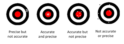
MSA studies the error within a measurement system. Measurement system error can be classified into three categories: accuracy, precision, and stability.

• Accuracy describes the difference between the measurement and the actual value of the part that is measured. It includes:
  • Bias: a measure of the difference between the true value and the observed value of a part. If the “true” value is unknown, it can be calculated by averaging several measurements with the most accurate measuring equipment available.
  • Linearity: a measure of how the size of the part affects the bias of a measurement system. It is the difference in the observed bias values through the expected range of measurement.
• Precision describes the variation you see when you measure the same part repeatedly with the same device. It includes the following two types of variation:
  • Repeatability: variation due to the measuring device. It is the variation observed when the same operator measures the same part repeatedly with the same device.
  • Reproducibility: variation due to the operators and the interaction between operator and part. It is the variation of the bias observed when different operators measure the same parts using the same device.
• Stability: a measure of how the accuracy and precision of the system perform over time.

The following picture illustrates accuracy and precision.

In this chapter, we will discuss how to conduct linearity and bias study and gage R&R (repeatability and reproducibility) analysis. The stability of a measurement system can be studied using statistical process control (SPC) charts.

Gage Linearity and Bias Study

Gage linearity tells you how accurate your measurements are across the expected range of the measurements. It answers the question, “Does my gage have the same accuracy for all sizes of objects being measured?”

Gage bias examines the difference between the observed average measurement and a reference value. It answers the question, “On average, how large is the difference between the values my gage yields and the reference values?”

Let’s use an example to show what linearity is.

Example of Linearity and Bias Study

If a baby is 8.5 lbs and the reading of a scale is 8.9 lbs, then the bias is 0.4 lb. If an adult is 85 lbs and the reading from the same scale is 85.4 lbs, then the bias is still 0.4 lb. This scale does not seem to have a linearity issue. However, if the reading for the adult were 89 lbs, the bias would seem to increase as the weight increases. Thus, you might suspect that the scale has a linearity issue.

The following data set shows measurements from a gage linearity and bias study.

Part	Reference	Reading	Part	Reference	Reading
1	2	1.95	3	6	6.04
1	2	2.10	3	6	6.25
1	2	2.00	3	6	6.21
1	2	1.92	3	6	6.16
1	2	1.97	3	6	6.06
1	2	1.94	3	6	6.03
1	2	2.02	4	8	8.40
1	2	2.05	4	8	8.35
1	2	1.95	4	8	8.15
1	2	2.04	4	8	8.10
2	4	4.09	4	8	8.18
2	4	4.16	5	10	10.49
2	4	4.16	5	10	10.28
2	4	4.10	5	10	10.42
2	4	4.06	5	10	10.29
2	4	4.11	5	10	10.14
2	4	4.02	5	10	10.07

The first column is the part ID. The second column is the “true” value of each part, called reference or master. In a linearity study, the selected reference should cover the minimal and maximal value of the produced parts. The Reading column is the observed value from a measurement device. Each part was measured multiple times, and some parts have the same reference value.

The following linear regression equation is used for gage linearity and bias study:

[math]\displaystyle{ Y={{\beta }_{0}}+{{\beta }_{1}}X+\varepsilon }[/math]

where:

• Y is the bias.
• X is the reference value.
• [math]\displaystyle{ {{\beta }_{0}} }[/math] and [math]\displaystyle{ {{\beta }_{1}} }[/math] are the coefficients.
• [math]\displaystyle{ \varepsilon }[/math] is error following a normal distribution
• [math]\displaystyle{ N\left( 0,{{\sigma }^{2}} \right) }[/math]

First, we need to calculate the bias for each observation in the above table. Bias is the difference between “Reading and Reference. The bias values are:

Part	Reference	Reading	Bias	Part	Reference	Reading	Bias
1	2	1.95	-0.05	3	6	6.04	0.04
1	2	2.1	0.1	3	6	6.25	0.25
1	2	2	0	3	6	6.21	0.21
1	2	1.92	-0.08	3	6	6.16	0.16
1	2	1.97	-0.03	3	6	6.06	0.06
1	2	1.94	-0.06	3	6	6.03	0.03
1	2	2.02	0.02	4	8	8.4	0.4
1	2	2.05	0.05	4	8	8.35	0.35
1	2	1.95	-0.05	4	8	8.15	0.15
1	2	2.04	0.04	4	8	8.1	0.1
2	4	4.09	0.09	4	8	8.18	0.18
2	4	4.16	0.16	5	10	10.49	0.49
2	4	4.16	0.16	5	10	10.28	0.28
2	4	4.1	0.1	5	10	10.42	0.42
2	4	4.06	0.06	5	10	10.29	0.29
2	4	4.11	0.11	5	10	10.14	0.14
2	4	4.02	0.02	5	10	10.07	0.07

Results for Linearity Study

Using the Reference column as X and the Bias column as Y in the linear regression, we get the following results:

Source of Variation	Degrees of Freedom	Sum of Squares [Partial]	Mean Squares [Partial]	F Ratio	P Value
Reference	1	0.3748	0.3748	40.4619	3.83E-07
Residual	32	0.2964	0.0093
Lack of Fit	3	0.01	0.0033	0.3388	0.7974
Pure Error	29	0.2864	0.0099
Total	33	0.6712

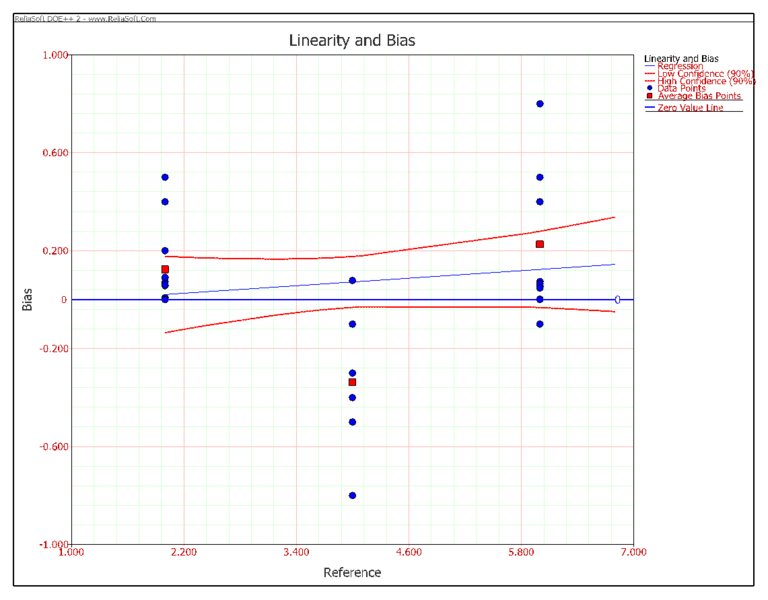
The calculated R-sq is 55.84% and R-sq(adj) is 54.46%. These values are not very high due to the large variation among the bias values. However, the p value of the lack of fit shows that the linear equation fits the data very well, and the following plot also shows there is a linear relation between reference and bias.

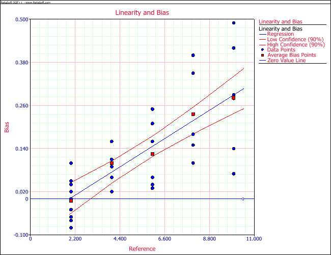
The estimated coefficients are:

Regression Information
Term	Coefficient	Standard Error	Low CI	High CI	T Value	P Value
Intercept	-0.0685	0.0347	-0.1272	-0.0098	-1.9773	0.0567
Reference	0.0358	0.0056	0.0263	0.0454	6.361	3.83E-07

The linearity is defined by:

[math]\displaystyle{ \begin{align} & \text{linearity}=|{{\beta }_{1}}|\times \text{process variation} \\ & \text{= }\!\!|\!\!\text{ }{{\beta }_{1}}|\times 6\times \text{process standard deviation} \end{align} }[/math]

This means that when this gage is used for a process, the observed process variation will be [math]\displaystyle{ |{{\beta }_{1}}| }[/math] times larger than the true process variation. This is because the observed value of a part is [math]\displaystyle{ |{{\beta }_{1}}| }[/math] times larger/smaller than the true value plus a constant value of the intercept.

The percentage of linearity (% linearity) is defined by:

[math]\displaystyle{ \text{ }\!\!%\!\!\text{ linearity}=100\left( \frac{\text{linearity}}{\text{process variation}} \right)%=\left( 100{{\beta }_{1}} \right)% }[/math]

% linearity shows the percentage of increase of the process variation due to the linearity of the gage. The smaller the linearity, the better the gage is.

If the linearity study shows no linear relation between reference and bias, you need to check the scatter plot of reference and bias to see if there is a non-linear relation. For example, the following plot shows a non-linear relationship between reference and bias.

Although the slope in the linear equation is almost 0 in the above plot, it does not mean the gage is accurate. The above figure shows an obvious V-shaped pattern between reference and bias. This non-linear pattern requires further analysis to judge whether the gage’s accuracy is acceptable.

Results for Bias Study

The bias study results are:

Reference	Bias	%Bias	Std of Mean	t	p
Average	0.1253	2.09%	0.017	7.3517	0.0000
2	-0.0060	0.10%	0.0183	0.3284	0.7501
4	0.1000	1.67%	0.0191	5.2223	0.0020
6	0.1250	2.08%	0.0385	3.2437	0.0229
8	0.2360	3.93%	0.0587	4.0203	0.0159
10	0.2817	4.70%	0.0652	4.3209	0.0076

• The Average row is the average of all the bias values while other rows are the reference values used in the study.

• The second column is the average bias for each reference value.

• The 3rd column is [math]\displaystyle{ |bias|/\text{process variation}\times \text{100 }\!\!%\!\!\text{ } }[/math]. Process variation is commonly defined as 6 times the process standard deviation. For this example, the process standard deviation is set to 1 and the process variation is 6.

• The 4th column is the standard deviation of the mean value of the bias for each reference value. If there are multiple parts having the same reference value, it is the pooled standard deviation of all the parts.

The T value is the ratio of the absolute value of the 2nd column and the 4th column. The p value is calculated from the T value and the corresponding degree of freedom for each reference value. If the p value is smaller than a given significance level, say 0.05, then the corresponding row has significant bias.

For this example, the p value column shows that bias appears for all the reference values except for the reference value of 2. The p value for Average row is very small, which means the average bias of all the readings is significant.

In some cases, such as the figure in the previous section, non-linearity occurs. Bias values are negative for some of the references and positive for others. Although each of the reference values can have significant bias, the average bias of all the references may not be significant.

When there are multiple parts for the same reference value, the standard deviation for that reference value is the pooled standard deviation of all the parts with the same reference value. The standard deviation for the average is calculated from the variance of all the parts.

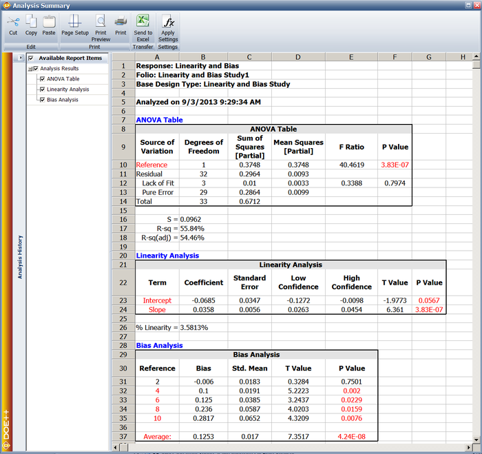
There are no clear cut-off values for what percent of linearity and bias are acceptable. Users should make their decision based on their engineering feeling or experience. The results from the Weibull++ DOE folio is given in the following picture.

Gage Repeatability and Reproducibility Study

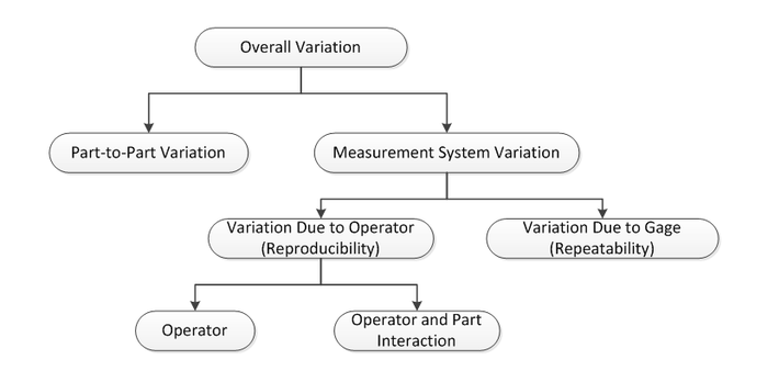
In the previous section, we discussed how to evaluate the accuracy of a measurement device by conducting a linearity and bias study. In this section, we will discuss how to evaluate the precision of a measurement device. Less variation means better precision. Gage repeatability and reproducibility (R&R) is a method for finding out the variations within a measurement system. Basically, there are 3 sources for variation: variation of the part, variation of the measurement device, and variation of operator. Variation caused by operator and interaction between operator and part is called reproducibility and variation caused by measurement device is called repeatability. The formal definitions of reproducibility and repeatability are given in the introduction of this chapter. In this section, we will briefly discuss how to calculate them. For more detail, please refer to Montgomery and Runger, 1993. The following picture shows the decomposition of variations for a product measured by a device.

Depending on how an experiment was conducted, there are two types of gage R&R study.

• When each part is measured multiple times by each operator, it is called a gage R&R crossed experiment.
• When each part is measured by only one operator, such as in destructive testing, this is called a gage R&R nested experiment.

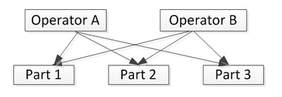
The following picture represents a crossed experiment.

In the above picture, operator A and operator B measured the same three parts. In a nested experiment, each operator measures different parts, as illustrated below.

The X-bar and R chart methods and the ANOVA method have been used to provide an estimation of the variance for each variation source in a measurements system. The X-bar and R chart methods cannot calculate the variance of operator by part interaction. In DOE++, we use the ANOVA method as discussed by Montgomery and Runger. The ANOVA method is the classical method for estimating variance components in designed experiments. It is more accurate than the X-bar and R chart methods.

In order to estimate variance, each part needs to be measured multiple times. For destructive testing, this is impossible. Therefore, some assumptions have to be made. Usually, for destructive testing, we need to assume that all the parts within the same batch are identical enough to claim that they are the same part. Nested design is the first option for destructive testing since each operator measures unique parts. If a part can be measured multiple times by different operators, then you would use crossed design.

From the above discussion, we know the total variability can be broken down into the following variance components:

[math]\displaystyle{ \begin{align} & \sigma _{total}^{2}=\sigma _{part}^{2}+\sigma _{gage}^{2} \\ & =\sigma _{part}^{2}+\left( \sigma _{repeatability}^{2}+\sigma _{reproducibility}^{2} \right) \\ & =\sigma _{part}^{2}+\left[ \sigma _{repeatability}^{2}+\left( \sigma _{operator}^{2}+\sigma _{operator\times part}^{2} \right) \right] \end{align} }[/math]

In practice, [math]\displaystyle{ 6{{\sigma }_{gauge}} }[/math] is called gage variation. It is compared to the specification or tolerance of the product measured using this gage to get the so called precision-to-tolerance ratio (or P/T ratio), as given by:

[math]\displaystyle{ \frac{P}{T}=\frac{6{{\sigma }_{gage}}}{USL-LSL} }[/math]

where USL and LSL are the upper and lower specification limits of the product under study.

If the P/T ratio is 0.1 or less, this implies adequate gage capability. There are obvious dangers in relying too much on the P/T ratio. For example, the ratio may be made arbitrarily small by increasing the width of the specification tolerance [AIAG]. Therefore, other ratios are also often used. One is the gage to part variation ratio:

[math]\displaystyle{ \frac{Gage}{Part}=\frac{{{\sigma }_{gage}}}{{{\sigma }_{part}}} }[/math]

The other is the gage to total variation ratio:

[math]\displaystyle{ \frac{Gage}{Total}=\frac{{{\sigma }_{gage}}}{{{\sigma }_{total}}} }[/math]

The smaller the above two ratios, the higher the relative precision of the gage is. The calculations for obtaining the above variance components for nested design and for crossed design are different.

We should be aware that gage R&R study should be conducted only when gage linearity and bias are not found to be significant.

Gage R&R Study for Crossed Experiments

From a design of experiment point of view, the experiment for gage R&R study is a general level 2 factorial design. Denoting the measurement by operator i on part j at replication k as [math]\displaystyle{ {{Y}_{ijk}} }[/math] , we have the following ANOVA model:

[math]\displaystyle{ {{Y}_{ijk}}=\mu +{{O}_{i}}+{{P}_{j}}+{{\left( OP \right)}_{ij}}+{{\varepsilon }_{kij}}\text{ }\left\{ \begin{align} & i=1,2,...,o; \\ & j=1,2,...,p; \\ & k=1,2,...,n \\ \end{align} \right. }[/math]

where:

• [math]\displaystyle{ {{O}_{i}} }[/math] is the effect of the ith operator.

• [math]\displaystyle{ {{P}_{j}} }[/math] is the effect of the jth operator.

• [math]\displaystyle{ {{\left( OP \right)}_{ij}} }[/math] represents the part and operator interaction.

• [math]\displaystyle{ {{\varepsilon }_{kij}} }[/math] is the random error that represents the repeatability.

Usually, all the effects in the above equation are assumed to be random effects that are normally distributed with mean of 0 and variance of [math]\displaystyle{ \sigma _{O}^{2} }[/math], [math]\displaystyle{ \sigma _{P}^{2} }[/math], [math]\displaystyle{ \sigma _{OP}^{2} }[/math], and [math]\displaystyle{ \sigma _{e}^{2} }[/math], respectively. When the operators in the study are the only operators who will work on the product, operator could be treated as fixed effect. However, as pointed out by Montgomery and Runger [], it is usually desirable to regard the operators as representatives of a larger operator population, with the specific operators having been randomly selected for the gage R&R study. Therefore, the operator should always be treated as a random effect. The definitions of fixed and random effects are:

• Fixed Effect: An effect associated with a factor that has a limited number of levels or in which only a limited number of levels are of interest to the experimenter.

• Random Effect: An effect associated with a factor chosen at random from a population having a large or infinite number of possible values.

A model that has only fixed effect factors is called a fixed effect model; a model that has only random effect factors is called a random effect model; a model that has both random and fixed effect factors is called a mixed effect model.

For random and mixed effect models, variance components can be estimated using least squares estimation, maximum likelihood estimation (MLE), and restricted MLE (RMLE) methods. The general calculations for variance components and F test in the ANOVA table are beyond the discussion of this chapter. For detail, readers are referred to Searl 1971 and 1997. However, when the design is balanced, variance components can be estimated using the regular linear regression method discussed in the general level factorial design chapter [1]. DOE++ uses this method for balanced designs.

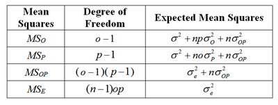
When a design is balanced, the expected mean squares for each effect in the above random effect model for gage R&R study using crossed design are:

The mean squares in the first column can be estimated using the model given at the beginning of this section. Their calculations are the same regardless of whether the model is fixed, random, or mixed. The difference for fixed, random, and mixed models is the expected mean squares. With the information in the above table, each variance component can be estimated by:

[math]\displaystyle{ \hat{\sigma }_{O}^{2}=\left( M{{S}_{O}}-M{{S}_{OP}} \right)/\left( pn \right) }[/math];

[math]\displaystyle{ \hat{\sigma }_{P}^{2}=\left( M{{S}_{P}}-M{{S}_{OP}} \right)/\left( on \right) }[/math];

[math]\displaystyle{ \hat{\sigma }_{OP}^{2}=\left( M{{S}_{OP}}-M{{S}_{e}} \right)/n }[/math]

[math]\displaystyle{ \hat{\sigma }_{e}^{2}=M{{S}_{E}} }[/math]

For the F test in the ANOVA table, the F ratio is calculated by:

[math]\displaystyle{ \left\{ \begin{align} & {{F}_{O}}=M{{S}_{O}}/M{{S}_{OP}}\text{ For operator} \\ & {{F}_{P}}=M{{S}_{P}}/M{{S}_{OP}}\text{ For part} \\ & {{F}_{OP}}=M{{S}_{OP}}/M{{S}_{E\text{ }}}\text{ For operator by part interaction} \\ \end{align} \right. }[/math]

From the above F ratio, we can test whether the effect of operator, part, and their interaction are significant or not.

Example: Gage R&R Study for Crossed Experiment

A gage R&R study was conducted using a crossed experiment. The data set is given in the table below. The product tolerance is 2,000. We want to evaluate the precision of this gage using the P/T ratio, gage to part variation ratio and gage to total variation ratio.

Part	Operator	Response
1	A	405
1	A	232
1	A	476
1	B	389
1	B	234
1	B	456
1	C	684
1	C	674
1	C	634
2	A	409
2	A	609
2	A	444
2	B	506
2	B	567
2	B	435
2	C	895
2	C	779
2	C	645
3	A	369
3	A	332
3	A	399
3	B	426
3	B	471
3	B	433
3	C	523
3	C	550
3	C	520

First, using the regular linear regression method, the mean square for each term can be calculated and is given in the following table.

Source of Variation	Degrees of Freedom	Sum of Squares [Partial]	Mean Squares [Partial]	F Ratio	P Value
Part	2	105545.00	52772.00	5.0655	0.0801
Operator	2	332414.00	166207.00	15.9538	0.0124
Part * Operator	4	41672.00	10418.00	1.4924	0.2462
Residual	18	125655.00	6980.85
Pure Error	18	125655.00	6980.85
Total	26	605285.00

All the effects are treated as random effects in the above table. The F ratios are calculated based on the equations given above. They are:

[math]\displaystyle{ \left\{ \begin{align} & {{F}_{O}}=M{{S}_{O}}/M{{S}_{OP}}=\text{166207/10418}=15.9538\text{ } \\ & {{F}_{P}}=M{{S}_{P}}/M{{S}_{OP}}=\text{52772/10418}=\text{5}\text{.0655 } \\ & {{F}_{OP}}=M{{S}_{OP}}/M{{S}_{E\text{ }}}=\text{10418/6981}=\text{1}\text{.4924} \\ \end{align} \right. }[/math]

The p value column shows that the operator is the most significant effect since that has the smallest p value. This means that the variation among all the operators is relatively large.

Second, based on the equations for expected mean squares, we can calculate the variance components. They are given in the following table.

Source	Variance	% Contribution
Part	4706.00	15.61%
Reproducibility	18455.60	61.23%
Operator	17309.89	57.43%
Operator*Part	1145.72	3.80%
Repeatability	6980.85	23.16%
Total Gage R&R	25436.46	84.39%
Total Variation	30142.46	100.00%

The above table shows:

[math]\displaystyle{ \hat{\sigma }_{O}^{2}=\left( M{{S}_{O}}-M{{S}_{OP}} \right)/\left( pn \right)=\frac{166207-10418}{3\times 3}=17309.89 }[/math]

[math]\displaystyle{ \hat{\sigma }_{P}^{2}=\left( M{{S}_{P}}-M{{S}_{OP}} \right)/\left( on \right)=\frac{52772-10418}{3\times 3}=4706.00 }[/math]

[math]\displaystyle{ \hat{\sigma }_{OP}^{2}=\left( M{{S}_{OP}}-M{{S}_{e}} \right)/n=\frac{10418-6981}{3}=1145.72 }[/math]

The repeatability is [math]\displaystyle{ \sigma _{e}^{2} }[/math] for the random error. The reproducibility is the sum of [math]\displaystyle{ \sigma _{O}^{2} }[/math] and [math]\displaystyle{ \sigma _{OP}^{2} }[/math]. The sum of repeatability and reproducibility is called the total gage R&R.

The last column in the above table shows the contribution of each variance component. For example, the contribution of the operator is 57.43%, which is calculated by:

[math]\displaystyle{ %\text{Contribution }\!\!\_\!\!\text{ Operator = 17309}\text{.89/30142}\text{.46=57}\text{.43 }\!\!%\!\!\text{ } }[/math]

The standard deviation for each effect is:

Source	Std (SD)
Part	68.600
Reproducibility	135.851
Operator	131.567
Operator*Part	33.848
Repeatability	83.551
Total Gage R&R	159.488
Total Variation	173.616

Since the product tolerance is 2,000, the P/T ratio is:

[math]\displaystyle{ \frac{P}{T}=\frac{6{{\sigma }_{gauge}}}{USL-LSL}=\frac{6\times 159.488}{2000}=47.85% }[/math]

Since P/T ratio is much greater than 10%, this gage is not adequate for this product.

The gage to part variation ratio:

[math]\displaystyle{ \frac{Gage}{Part}=\frac{{{\sigma }_{gage}}}{{{\sigma }_{part}}}=\frac{159.488}{68.600}=232.49% }[/math]

The gage to total variation ratio:

[math]\displaystyle{ \frac{Gage}{Total}=\frac{{{\sigma }_{gage}}}{{{\sigma }_{total}}}=\frac{159.488}{173.616}=91.86% }[/math]

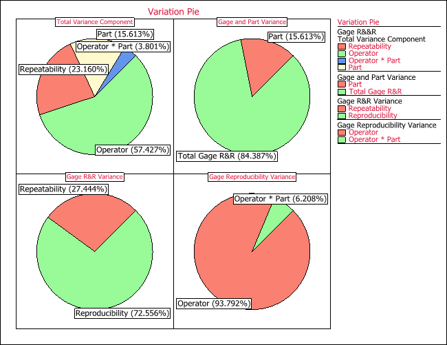
Clearly, all the ratios are too large. The operators should be trained and a new gage may need to be purchased. The pie chart plots for the contribution of each variance components are shown next.

In the above picture, the total variation component pie chart displays the ratio of each variance to the total variance. The gage and part variation chart displays the ratio of the gage variance to the total variance, and the ratio of the part to the total variance. The gage R&R variance is for the percentage of repeatability and reproducibility to the total gage variance. The gage reproducibility variance pie chart future decomposes reproducibility to operator variance, and operator and part interaction variance.

Gage R&R Study for Nested Experiments

When the experiment is nested, since the part is nested within each operator, we cannot assess the operator and part interaction. The regression model is:

[math]\displaystyle{ {{Y}_{ijk}}=\mu +{{O}_{i}}+{{P}_{j(i)}}+{{\varepsilon }_{kij}}\text{ }\left\{ \begin{align} & i=1,2,...,o; \\ & j=1,2,...,p; \\ & k=1,2,...,n \\ \end{align} \right. }[/math]

The estimated operator effect includes the operator effect and the operator and part interaction. For the general calculation on the above model, please refer to [“Applied Linear Statistical Models” by Kutner, Nachtsheim, Neter and Li]. When the nested experiment is balanced, its calculations for total sum of squares (SST), sum of squares of operator (SSO), and sum of square of error (SSE) are the same as those for the crossed design. The only difference is the sum of squares of part (SSP(O)). For nested designs, it is:

[math]\displaystyle{ S{{S}_{P(O)}}=S{{S}_{P}}+S{{S}_{OP}} }[/math]

SSP and SSOP are the sum of squares for part, and the sum of squares for part and operator interaction. They are calculated using a linear regression equation by including part and operator interaction in the model.

When the design is balanced, the expected mean squares for each effect in the above random effect model for gage R&R study nested design are:

Mean Squares	Degree of Freedom	Expected Mean Squares
MSO	[math]\displaystyle{ o-1 }[/math]	[math]\displaystyle{ {{\sigma }^{2}}+np\sigma _{O}^{2}+n\sigma _{P(O)}^{2} }[/math]
MSP(O)	[math]\displaystyle{ o(p-1) }[/math]	[math]\displaystyle{ {{\sigma }^{2}}+n\sigma _{P(O)}^{2} }[/math]
MSE	[math]\displaystyle{ (n-1)op }[/math]	[math]\displaystyle{ \sigma _{e}^{2} }[/math]

With the information in the above table, each variance component can be estimated by:

[math]\displaystyle{ \hat{\sigma }_{O}^{2}=\left( M{{S}_{O}}-M{{S}_{P(O)}} \right)/\left( pn \right) }[/math];

[math]\displaystyle{ \hat{\sigma }_{P(O)}^{2}=\left( M{{S}_{P(O)}}-M{{S}_{E}} \right)/n }[/math];

[math]\displaystyle{ \hat{\sigma }_{e}^{2}=M{{S}_{E}} }[/math]

For the F test in the ANOVA table, the F ratio is calculated by:

[math]\displaystyle{ \left\{ \begin{align} & {{F}_{O}}=M{{S}_{O}}/M{{S}_{P(O)}}\text{ For operator} \\ & {{F}_{P(O)}}=M{{S}_{P}}/M{{S}_{E}}\text{ For part (nested in operator)} \\ \end{align} \right. }[/math]

Example: Gage R&R Study for Nested Experiment

For the example in the previous section, since it is a nested design, the part i measured by one operator is different from the part i measured by another operator. Therefore, when the design is nested, the design in fact should be:

Part	Operator	Response
1_1	A	405
1_1	A	232
1_1	A	476
2_1	B	389
2_1	B	234
2_1	B	456
3_1	C	684
3_1	C	674
3_1	C	634
1_2	A	409
1_2	A	609
1_2	A	444
2_2	B	506
2_2	B	567
2_2	B	435
3_2	C	895
3_2	C	779
3_2	C	645
1_3	A	369
1_3	A	332
1_3	A	399
2_3	B	426
2_3	B	471
2_3	B	433
3_3	C	523
3_3	C	550
3_3	C	520

We want to evaluate the precision of this gage using the P/T ratio, gage to part variation ratio, and gage to total variation ratio.

First, using the regular linear regression method for nested designs [Neter’s book], all the mean squares for each term can be calculated. They are given in the following table.

Source of Variation	Degrees of Freedom	Sum of Squares [Partial]	Mean Squares [Partial]	F	P
Operator	2	332414.00	166207.00	6.77396	0.028917
Part(Operator)	6	147217.00	24536.17	3.514781	0.017648
Residual	18	125655.00	6980.85
Pure Error	18	125655.00	6980.85
Total	26	605285.00

The F ratios are calculated based on the equations given above.

[math]\displaystyle{ \left\{ \begin{align} & {{F}_{O}}=M{{S}_{O}}/M{{S}_{P(O)}}\text{ }=\text{166207/24536}\text{.17}=\text{6}\text{.774} \\ & {{F}_{P(O)}}=M{{S}_{P}}/M{{S}_{E}}=\text{24536}\text{.17/6980}\text{.85}=\text{3}\text{.515} \\ \end{align} \right. }[/math]

The p value column shows that the operator and part (operator) both are significant at a significance level of 0.05.

Second, based on the equations for expected mean squares, we can calculate the variance components. They are given in the following table.

Source	Variance	% Contribution
Repeatability	6981	24.43%
Reproducibility	15741.2037	55.09%
Operator	15741.2037	55.09%
Part (Operator)	5851.7716	20.48%
Total Gage R&R	22722	79.52%
Total Variation	28574	100.00%

The standard deviation for each variation source is:

Source	Std (SD)
Repeatability	83.551
Reproducibility	125.464
Operator	125.464
Part (Operator)	76.497
Total Gage R&R	150.738
Total Variation	169.038

Since the product tolerance is 2,000, the P/T ratio is:

[math]\displaystyle{ \frac{P}{T}=\frac{6{{\sigma }_{gage}}}{USL-LSL}=\frac{6\times 150.738}{2000}=45.22% }[/math]

Since the P/T ratio is much greater than 10%, this gage is not adequate for this product.

The gage to part variation ratio:

[math]\displaystyle{ \frac{Gage}{Part}=\frac{{{\sigma }_{gage}}}{{{\sigma }_{part(operator)}}}=\frac{150.738}{76.497}=197.05% }[/math]

The gage to total variation ratio:

[math]\displaystyle{ \frac{Gage}{Total}=\frac{{{\sigma }_{gage}}}{{{\sigma }_{total}}}=\frac{150.738}{169.038}=89.17% }[/math]

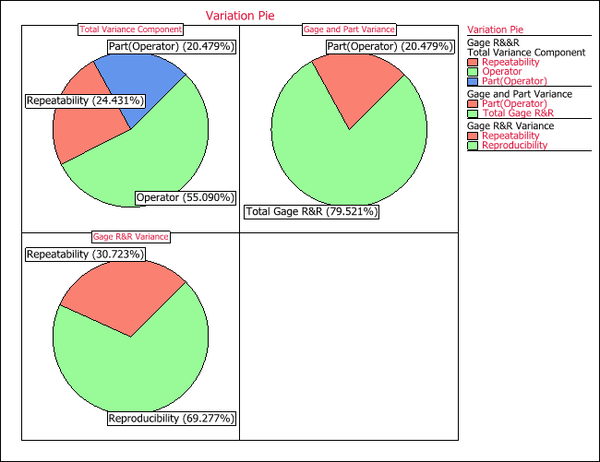
The pie charts for all the variance components are shown next.

X-bar and R Charts in Gage R&R

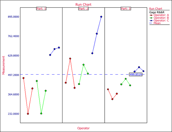
X-bar and R charts are often used in gage R&R studies. Although DOE++ does not use them to estimate repeatability and reproducibility, they are included in the plot to visually display the data. Along with X-bar and R charts, other plots are also used in DOE++. For example, the following is a run chart for the example of gage R&R study using crossed design.

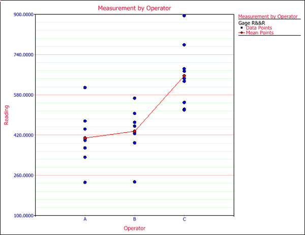
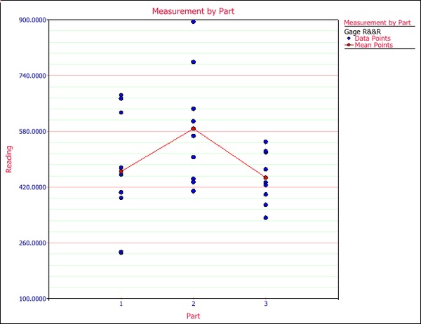
Each column in the above figure is the 9 measurements of a part by all the operators. In the above plot, we see that all readings by operator C (the blue points) are above the mean line. This indicates that operator C’s readings are different from the calculated mean. Part 3 (the last column in the plot) has the least variation among these 3 parts. These two conclusions also can be inferred from the following two plots.

The above plot shows that operator C’s readings are much higher than the other two operators.

The above plot shows part 3 has less variation compared to parts 1 and 2.

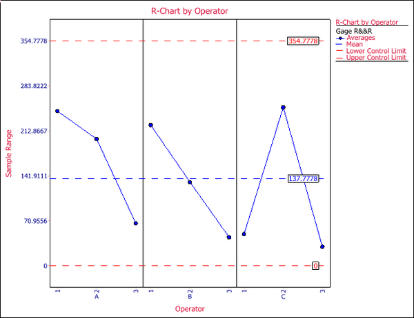
Now let’s talk about X-bar and R charts. The X-bar chart is used to see how the mean reading changes among the parts; the R chart is used to check the repeatability. When the number of readings of each part by the same operator is greater than 10, an s chart is used to replace the R chart. The R chart is accurate only when the sample size is small (<10). For this example, the sample size is 3, so the R chart is used, as shown next.

In the above plot, the x-axis is operator and the y-axis is the range for each part measured by each operator.

The step-by-step calculation for the R chart (n [math]\displaystyle{ \le }[/math]10) is given below.

Step 1: calculate the range of each part for each operator.

[math]\displaystyle{ {{R}_{i,j}}=\max ({{X}_{ijk}})-\min \left( {{X}_{ijk}} \right) }[/math]

[math]\displaystyle{ {{R}_{i,j}} }[/math] is the range of the reading for the ith part and the jth operator. k is the trial number.

Step 2: calculate the average range for each operator.

[math]\displaystyle{ {{\bar{R}}_{j}}=average({{R}_{i,j}}) }[/math]

Step 3: calculate the overall average range for all the operators.

[math]\displaystyle{ \bar{\bar{R}}=average({{\bar{R}}_{j}}) }[/math]

This is the central line in the R chart.

Step 4: calculate the upper control limit (UCL) and the lower control limit (LCL) for the R chart.

[math]\displaystyle{ \begin{align} & UCL=D4*\bar{\bar{R}}; \\ & LCL=D3*\bar{\bar{R}} \\ \end{align} }[/math]

D3 and D4 are from the following table:

n	A2	D3	D4	d2
2	1.88	0	3.267	1.128
3	1.023	0	2.575	1.693
4	0.729	0	2.282	2.059
5	0.577	0	2.115	2.326
6	0.483	0	2.004	2.534
7	0.419	0.076	1.924	2.704
8	0.373	0.136	1.864	2.847
9	0.337	0.184	1.816	2.97
10	0.308	0.223	1.777	3.078

The calculation results for this example are:

	Operator A
Part Number	T1	T2	T3	[math]\displaystyle{ {{\bar{R}}_{ij}} }[/math]	[math]\displaystyle{ {{\bar{X}}_{ij}} }[/math]	[math]\displaystyle{ {{\bar{X}}_{j}} }[/math]
1	405	232	476	244	371
2	409	609	444	200	487.3333	408.3333
3	369	332	399	67	366.6667
	Operator B
1	389	234	456	222	359.6667
2	506	567	435	132	502.6667	435.2222
3	426	471	433	45	443.3333
	Operator C
1	684	674	634	50	664
2	895	779	645	250	773	656
3	523	550	520	30	531
			[math]\displaystyle{ \bar{\bar{R}} }[/math]	137.7778	[math]\displaystyle{ \bar{\bar{X}} }[/math]	499.8519

From the above table, we know that the three values for the R chart are:

[math]\displaystyle{ \begin{align} & UCL=D4*\bar{\bar{R}}=2.575\times 137.778=354.7784 \\ & \bar{\bar{R}}=137.7778 \\ & LCL=D3*\bar{\bar{R}}=0 \\ \end{align} }[/math]

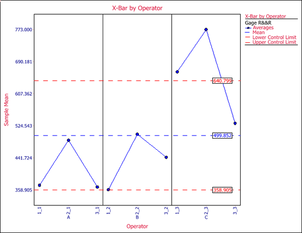
The step by step calculation for the X-bar chart for sample size n, where n is less than or equal to 10, is given below.

Step 1: Calculate the average of the reading for part i, by operator j.

[math]\displaystyle{ {{\bar{X}}_{ij}}=average\left( {{X}_{ijk}} \right) }[/math]

Step 2: Calculate the overall mean of operator j.

[math]\displaystyle{ {{\bar{X}}_{j}}=average\left( {{{\bar{X}}}_{ij}} \right) }[/math]

Step 3: Calculate the overall mean of all the observations:

[math]\displaystyle{ \bar{\bar{X}}=average({{\bar{X}}_{j}}) }[/math]

[math]\displaystyle{ \bar{\bar{X}} }[/math] is the central line of the X-bar chart.

The above table gives the values of [math]\displaystyle{ {{\bar{X}}_{ij}} }[/math], [math]\displaystyle{ {{\bar{X}}_{j}} }[/math], and [math]\displaystyle{ \bar{\bar{X}} }[/math].

Step 4: Calculate the UCL and LCL.

[math]\displaystyle{ UCL=\bar{\bar{X}}+A2*\bar{\bar{R}} }[/math]

[math]\displaystyle{ LCL=\bar{\bar{X}}-A2*\bar{\bar{R}} }[/math]

A2 is from the above constant value table. The X-bar chart for this example is:

When the sample size (the reading of the same part by the same operator) is greater than 10, the more accurate s chart is used to replace the R chart. The calculation for the UCL and LCL in the X-bar chart is also updated using the sample standard deviation s.

The step by step calculations for the s chart are given below.

Step 1: Calculate the standard deviation for each part of each operator.

[math]\displaystyle{ {{S}_{ij}}=\frac{1}{n-1}\sum\limits_{k}^{{}}{\left( {{x}_{ijk}}-{{{\bar{x}}}_{ij}} \right)} }[/math]

Step 2: Calculate the average of these standard deviations.

[math]\displaystyle{ \bar{S}=average({{S}_{ij}}) }[/math]

The above equation is only valid for balanced designs.

[math]\displaystyle{ \bar{S} }[/math] is the central line for the s chart.

Step 3: Calculate the UCL and LCL.

[math]\displaystyle{ UCL=\bar{S}+3\frac{{\bar{S}}}{{{c}_{4}}}\times {{c}_{5}} }[/math]; [math]\displaystyle{ LCL=\bar{S}-3\frac{{\bar{S}}}{{{c}_{4}}}\times {{c}_{5}} }[/math]

where:

[math]\displaystyle{ {{c}_{4}}=\sqrt{\frac{2}{n-1}}\frac{\left( \frac{n}{2}-1 \right)!}{\left( \frac{n-1}{2}-1 \right)!}={{\left( \frac{2}{n-1} \right)}^{1/2}}\frac{\Gamma (n/2)}{\Gamma (\frac{n-1}{2})} }[/math];

[math]\displaystyle{ {{c}_{5}}=\sqrt{1-c_{4}^{2}} }[/math]

For the X-bar chart, the central line is the same as before. Only the UCL and LCL need to use the following equations when n>10.

[math]\displaystyle{ UCL=\bar{\bar{x}}+3\frac{{\bar{S}}}{{{c}_{4}}\sqrt{n}} }[/math];

[math]\displaystyle{ UCL=\bar{\bar{x}}-3\frac{{\bar{S}}}{{{c}_{4}}\sqrt{n}} }[/math]

From the above calculation, it can be seen the calculation for the s chart is much more complicated than the calculation for the R chart. This is why the R chart was often used in the past, before computers were in common use.

Gage Agreement Study

In the above sections, we discussed how to evaluate a gage’s accuracy and precision. Accuracy is assessed using a linearity and bias study, while precision is evaluated using a gage R&R study. Often times, we need to compare two measurement devices. For instance, can an old device be replaced by a new one, or can an expensive one be replaced by a cheap one, without loss of the accuracy and precision of the measurements? The study used for comparing the accuracy and precision of two gages is called a gage agreement study.

Accuracy Agreement Study

One way to compare the accuracy of two gages is to conduct a linearity and bias study for each gage by the same operator, and then compare the percentages of the linearity and bias. This provides a rough idea of how close the accuracies of the two gages are. However, it is difficult to quantify how close they should be in order to claim there is no significant difference between them. Therefore, a formal statistical method is needed. Let’s use the following example to explain how to compare the accuracy of two devices.

Example: Compare the Accuracy of Two Gages Using a Paired t-Test

There are two gages: Gage 1 and Gage 2. There are 17 subjects/parts. For each subject, there are two readings from each gage.

	Gage 1		Gage 2
Subject	1st Reading	2nd Reading	1st Reading	2nd Reading
1	494	490	512	525
2	395	397	430	415
3	516	512	520	508
4	434	401	428	444
5	476	470	500	500
6	557	611	600	625
7	413	415	364	460
8	442	431	380	390
9	650	638	658	642
10	433	429	445	432
11	417	420	432	420
12	656	633	626	605
13	267	275	260	227
14	478	492	477	467
15	178	165	259	268
16	423	372	350	370
17	427	421	451	443

If their bias and linearity are the same, then the difference between the average readings for the same subject by the two devices should be almost the same. In other words, the differences should be around 0, with a constant standard deviation. We can test if this hypothesis is true or not. The differences of the readings are given in the table below.

Subject	Gage 1		Gage 2		Difference	Grand Average
	Number of Reading	Average Reading	Number of Reading	Average Reading
1	2	492	2	518.5	-26.5	505.25
2	2	396	2	422.5	-26.5	409.25
3	2	514	2	514	0	514
4	2	417.5	2	436	-18.5	426.75
5	2	473	2	500	-27	486.5
6	2	584	2	612.5	-28.5	598.25
7	2	414	2	412	2	413
8	2	436.5	2	385	51.5	410.75
9	2	644	2	650	-6	647
10	2	431	2	438.5	-7.5	434.75
11	2	418.5	2	426	-7.5	422.25
12	2	644.5	2	615.5	29	630
13	2	271	2	243.5	27.5	257.25
14	2	485	2	472	13	478.5
15	2	171.5	2	263.5	-92	217.5
16	2	397.5	2	360	37.5	378.75
17	2	424	2	447	-23	435.5

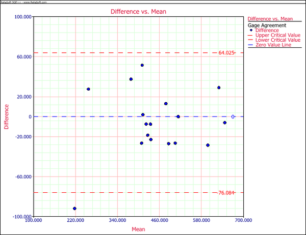
The difference vs. mean plot is shown next.

Difference vs Mean plot for gage agreement study

The above plot shows that all the values are within the control limits (significant level = 0.05) except for one point, and are evenly distributed around the central 0 line.

The paired t-test is used to test if the two gages have the same bias (i.e., if the “difference” has a mean value of 0). The paired t-test is conducted using the Difference column. The calculation is given below.

Step 1: Calculate the mean value of this column.

[math]\displaystyle{ \bar{x}=\frac{1}{n}\sum\limits_{i=1}^{n}{{{x}_{i}}} }[/math]

For this example, n is 17.

Step 2: Calculate the standard deviation of this column.

[math]\displaystyle{ Var(x)=\frac{1}{n-1}\sum\limits_{i=1}^{n}{{{\left( {{x}_{i}}-\bar{x} \right)}^{2}}} }[/math]

[math]\displaystyle{ Std(x)=\sqrt{Var(x)} }[/math]

Step 3: Conduct the t-test.

[math]\displaystyle{ {{t}_{0}}=\frac{{\bar{x}}}{std(x)/\sqrt{n}} }[/math]

Step 4: Calculate the p value.

[math]\displaystyle{ p=InvT(df=n-1,{{t}_{0}}) }[/math]

The calculation will be summarized in the following table.

Mean (Gage 1- Gage 2)	Std. Mean	Lower Bound	Upper Bound	T Value	P Value
6.02941	8.053186092	-23.101404	11.04257999	0.748698924	0.464904

Since the p value is 0.464904, which is greater than the significant level of 0.05, the two gages have the same bias.

The paired t-test is valid only when there is no trend or pattern in the difference vs. mean plot. If the points show a pattern such as a linear pattern, the conclusion from the paired t-test may not be valid.

Example: Compare the Accuracy of Two Gages Using Linear Regression

The data set for a gage agreement study is given in the table below.

Subject	Gage 1		Gage 2
	1st Reading	2nd Reading	1st Reading	2nd Reading
1	66.32	65.80	74.30	74.39
2	95.51	95.94	94.74	94.93
3	61.93	60.27	70.81	70.75
4	163.08	162.33	149.91	149.75
5	76.60	76.56	82.00	81.53
6	127.35	127.68	120.58	120.70
7	93.07	90.51	92.96	92.88
8	134.39	134.49	126.24	126.23
9	115.54	114.33	112.27	112.96
10	117.92	118.26	112.41	113.18

The differences of the readings are given in the table below.

Subject	Gage 1		Gage 2		Difference	Grand Average
	Number of Reading	Average Reading	Number of Reading	Average Reading
1	2	66.06	2	74.35	-8.29	70.20
2	2	95.72	2	94.83	0.89	95.28
3	2	61.10	2	70.78	-9.67	65.94
4	2	162.70	2	149.83	12.87	156.26
5	2	76.58	2	81.77	-5.19	79.17
6	2	127.52	2	120.64	6.88	124.08
7	2	91.79	2	92.92	-1.13	92.35
8	2	134.44	2	126.24	8.20	130.34
9	2	114.94	2	112.61	2.32	113.77
10	2	118.09	2	112.79	5.30	115.44

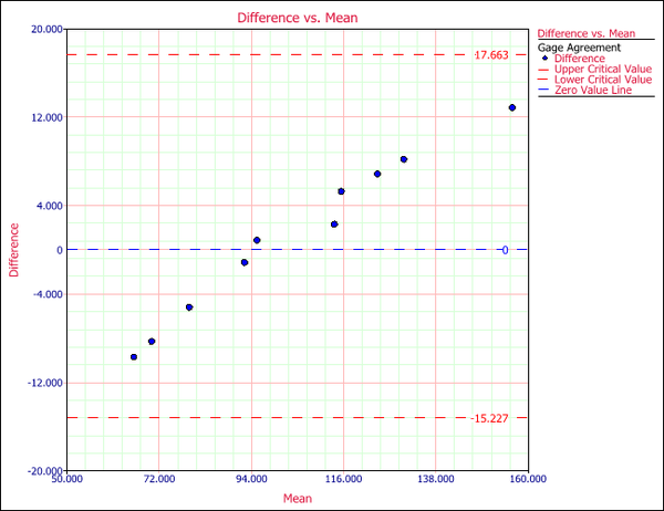
The difference vs. mean plot shows a clear linear pattern, although all the points are within the control limits.

Difference vs Mean plot for gage agreement study with a linear trend

The paired t-test results are:

Mean (Gage 1- Gage 2)	Std. Mean	Lower Bound	Upper Bound	T Value	P Value
1.218	7.3804	17.9137	-15.4777	0.5219	0.6144

Since the p value is large, we cannot reject the null hypothesis. The conclusion is that the bias is the same for these two gages. However, the linear pattern in the above plot makes us suspect that this conclusion may not be accurate. We need to compare both the bias and the linearity. The F-test used in linear regression can do the work.

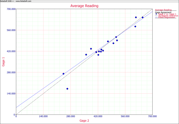
If the two gages have the same accuracy (linearity and bias), then the average readings from Gage 1 and the average readings from Gage 2 should be on a 45 degree line that passes the origin in the average reading plot. However, the following plot shows the points are not very close to the 45 degree line.

Average readings comparison

We can fit a linear regression equation:

[math]\displaystyle{ Y={{\beta }_{0}}+{{\beta }_{1}}X+\varepsilon }[/math]

where Y is the average reading for each part from Gage 1, and X is the average reading for each part from Gage 2. If the two gages agree with each other, then [math]\displaystyle{ {{\beta }_{0}} }[/math] should be 0 and [math]\displaystyle{ {{\beta }_{1}} }[/math] should be one. Using the data in this example, the calculated regression coefficients are:

Term	Coefficient	Standard Error	Low Confidence	High Confidence	T Value	P Value
[math]\displaystyle{ {{\beta }_{0}} }[/math]	22.3873	1.2471	19.5114	25.2633	17.9508	9.51E-08
[math]\displaystyle{ {{\beta }_{1}} }[/math]	0.775	0.0114	0.7487	0.8013	19.7265	4.54E-08

The p values in the above results show that [math]\displaystyle{ {{\beta }_{0}} }[/math] is not 0 and [math]\displaystyle{ {{\beta }_{1}} }[/math] is not 1. These tests are for each individual coefficient. For [math]\displaystyle{ {{\beta }_{0}} }[/math], the t value is:

[math]\displaystyle{ {{t}_{0}}=\frac{\left| {{\beta }_{0}} \right|}{1.2471}=17.9508 }[/math]

For [math]\displaystyle{ {{\beta }_{1}} }[/math], the t value is

[math]\displaystyle{ {{t}_{1}}=\frac{\left| {{\beta }_{1}}-1 \right|}{0.0114}=19.7265 }[/math]

The p value is calculated using the above t values and the degree of freedom of error of 8.

Since we want to test these two coefficients simultaneously, using an F-test is more appropriate. The null hypothesis for the F-test is:

[math]\displaystyle{ \begin{align} & H0:\text{ (}{{\beta }_{0}},{{\beta }_{1}})=(0,1) \\ & H1:\text{(}{{\beta }_{0}},{{\beta }_{1}})\ne (0,1) \\ \end{align} }[/math]

Under the null hypothesis, the statistic is:

[math]\displaystyle{ f=\frac{\left[ \text{(}{{{\hat{\beta }}}_{0}},{{{\hat{\beta }}}_{1}})-(0,1) \right]{{\Sigma }^{-1}}\left[ \text{(}{{{\hat{\beta }}}_{0}},{{{\hat{\beta }}}_{1}})-(0,1) \right]'}{2}\tilde{\ }F(2,dfErr) }[/math]

For this example:

[math]\displaystyle{ f=200.5754 }[/math]

The result for the F-test is given below.

Simultaneous Coefficient Test
Test	F Value	P Value
[math]\displaystyle{ {{\beta }_{0}} }[/math]= 0 and [math]\displaystyle{ {{\beta }_{1}} }[/math]= 1	200.5754	3.43E-08

Since the p value is almost 0 in the above table, we have enough evidence to reject the null hypothesis. Therefore, these two gages have different accuracy.

This example shows that the paired t-test and the regression coefficient test give different conclusion. This is because the t-test cannot catch the difference between the linearity of these two gages, while the simultaneous regression coefficient test can.

Precision Agreement Study

A gage agreement experiment should be conducted by the same operator, so the gage reproducibility caused by operator is removed. Only repeatability caused by gages is calculated and compared. Therefore precision agreement study is comparing the repeatability of each gage. Let’s use the first example in the above accuracy agreement study for a precision agreement study.

First, we need to calculate the repeatability of each gage. Repeatability is also the pure error which is the variation of the multiple readings for the same part by the same operator. The result of Gage 2 is given in the following table.

Subject	1st Reading	2nd Reading	Sum of Square (SS)
1	512	525	84.5
2	430	415	112.5
3	520	508	72
4	428	444	128
5	500	500	0
6	600	625	312.5
7	364	460	4608
8	380	390	50
9	658	642	128
10	445	432	84.5
11	432	420	72
12	626	605	220.5
13	260	227	544.5
14	477	467	50
15	259	268	40.5
16	350	370	200
17	451	443	32
		Total SS	6739.5
		Repeatability	396.4412

The repeatability is calculated by the following steps.

Step 1: For each subject, calculate the sum of square (SS) of the repeated readings for the same gage. For example, for subject 1, the SS under this gage is:

[math]\displaystyle{ S{{S}_{i}}=\sum\limits_{i=1}^{{{n}_{i}}}{({{x}_{i}}-\bar{x})_{{}}^{2}}=\left[ {{\left( 512-518.5 \right)}^{2}}+{{\left( 525-518.5 \right)}^{2}} \right]=84.5 }[/math]

Step 2: Add the SS of all the subjects together.

[math]\displaystyle{ }[/math][math]\displaystyle{ SS=\sum\limits_{i=1}{S{{S}_{i}}} }[/math]

Step 3: Find the degree of freedom.

[math]\displaystyle{ df=\sum\limits_{i=1}^{n}{({{n}_{i}}-1)} }[/math]

[math]\displaystyle{ {{n}_{i}} }[/math] is the number of repeated reading for subject i. n is the total number of subjects.

Step 4: Calculate the variance (repeatability). For Gage 2, it is:

[math]\displaystyle{ \hat{s}_{2}^{2}=\frac{SS}{df}=396.4412 }[/math]

Repeating the above procedure, we can get the repeatability for gage 1. It is 234.2941. We can then compare the repeatability of these two gages. If these two variances are the same, then the ratio of them follows an F distribution with degree of freedom of [math]\displaystyle{ d{{f}_{1}} }[/math] and [math]\displaystyle{ d{{f}_{2}} }[/math]. [math]\displaystyle{ d{{f}_{1}} }[/math] is the degree of freedom for Gage 1 (the numerator in the F ratio) and Gage 2 (the denominator in the F ratio).

The results are:

Gage	Repeatability Variance	Degrees of Freedom	F Ratio	Lower Bound	Upper Bound	P Value
Gage 1	234.2941	17	0.591	0.22101	1.5799	0.1440
Gage 2	396.4412	17

The p value in the range of (risk level)/2 = 0.025 and 1-(risk level)/2 = 0.975. Therefore, we cannot reject the null hypothesis that these two gages have the same precision.

The bounds in the above table are calculated by:

[math]\displaystyle{ {f_U}=invF(d{{f}_{1}},d{{f}_{2}},\alpha /2) }[/math]

[math]\displaystyle{ {f_L}=invF(d{{f}_{1}},d{{f}_{2}},1-\alpha /2) }[/math]

[math]\displaystyle{ \text{Upper bound}={{F}_{ratio}}/{{f}_{L}} }[/math]

[math]\displaystyle{ \text{Lower bound}={{F}_{ratio}}/{{f}_{U}} }[/math]

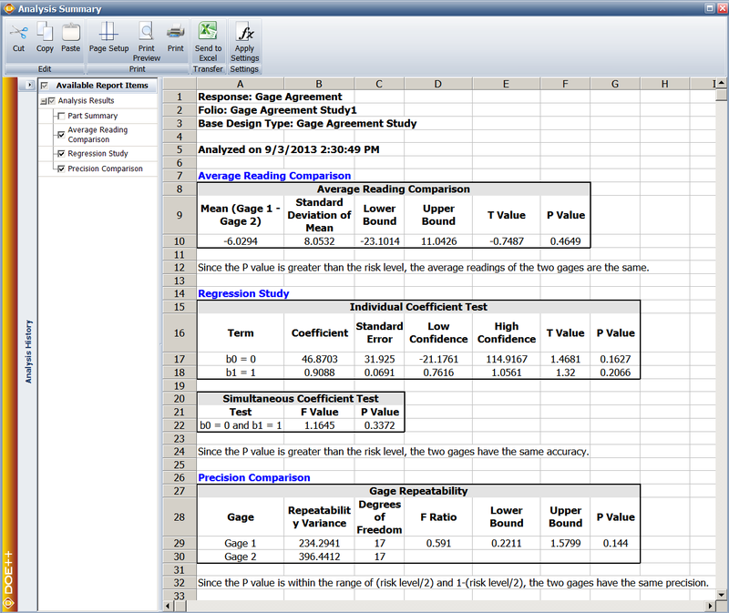
For this example [math]\displaystyle{ {f_U}=2.6733 }[/math] and [math]\displaystyle{ {{f}_{L}}=0.374069 }[/math]. Therefore, the upper bound is 1.5799 and the lower bound is 0.22101. Since the bounds include 1, it means the two gages have the same repeatability. The results from DOE++ are given below.

Gage agreement study results from DOE++

General Guidelines on Measurement System Analysis

The experiments for MSA should be designed experiments. The experiment should be designed and conducted based on DOE principals. Here are some of the guidelines for preparation prior to conducting MSA [AIAG].

1. Whenever possible, the operators chosen should be selected from those who normally operate the gage. If these operators are not available, then personnel should be properly trained in the correct usage of the gage.
2. The sample parts must be selected from the process which represents its entire operating range. This is sometimes done by taking one sample per day for several days. The collected samples will be treated as if they represent the full range of product variation. Each part must be numbered for identification.
3. The gage must have a graduation that allows at least one-tenth of the expected process variation of the characteristic to be read directly. Process variation is usually defined as 6 times the process standard deviation. For example, if the process variation is 0.1, the equipment should read directly to an increment no larger than 0.01.

The manner in which a study is conducted is very important if reliable results are to be obtained. To minimize the possibility of getting inaccurate results, the following steps are suggested:

1. The measurements should be made in a random order. The operators should be unaware of which numbered part is being checked in order to avoid any possible bias. However, the person conducting the study should know which numbered part is being checked and record the data accordingly, such as Operator A, Part 1, first trial.
2. In reading the gage, the readings should be estimated to the nearest number that can be obtained. At a minimum, readings should be made to one-half of the smallest graduation. For example, if the smallest graduation is 0.01, then the estimate for each reading should be rounded to the nearest 0.005.