RGA Data Types
Reliability growth analysis can be conducted using different data types. This chapter explores and examines the possible data schemes, and outlines the available models for each data type. The data types for developmental testing (traditional reliability growth analysis) will be discussed first. Then we will discuss the data types that support the use of RGA models for analyzing fielded systems (either for repairable systems analysis or fleet data analysis).
Developmental Testing Data Types
Time-to-Failure Data
Time-to-failure (continuous) data is the most commonly observed type of reliability growth data. It involves recording the times-to-failure for the unit(s) under test. Time-to-failure data can be applied to a single unit or system or to multiple units or systems. There are multiple data entry schemes for this data type and each is presented next.
Failure Times Data
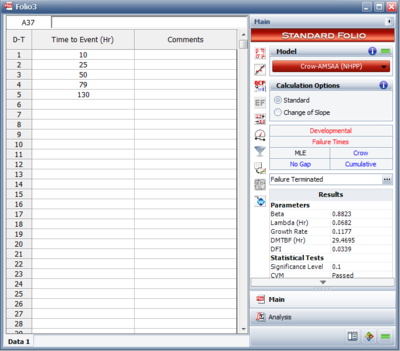
This data type is used for tests where the actual system failure times are tracked and recorded. The data can be entered in a cumulative format (where each row shows the total amount of test time) or non-cumulative format (where each row shows the incremental test time), as shown next.
Grouped Failure Times
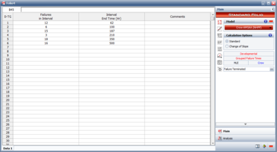
This data type is used for tests where the exact failure times are unknown and only the number of failures within a time interval are recorded (e.g., inspection data). For a single system, multiple failures can occur before the operator stops the test. In this case, X number of failures are found after Y hours of test time. Failures [math]\displaystyle{ X_{1}\,\! }[/math], [math]\displaystyle{ X_{2}\,\! }[/math], [math]\displaystyle{ X_{3}\,\! }[/math], etc. could have occurred at any time period up to the termination time, thus exact times for each failure are not available. This is commonly called interval or grouped data. Grouped data can be helpful to merge data from multiple locations.
When multiple units are tested, the units are inspected at predetermined time intervals and the number of failed units is recorded. When entering the time at which the failures occurred for grouped data, the time is equal to the total accumulated test time for all of the units being tested. The number of failed units is simply equal to the number of failures that occurred during the current interval. The next figure shows an example of data entry for grouped data.
Assumptions:
- Intervals do not have to be of equal length.
- All units within each interval should be the same configuration. However, the number of units does not have to be the same.
Multiple Systems (Known Operating Times)
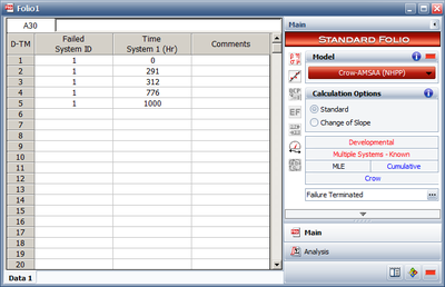
This data type is used for tests where a number of systems are tested, and if a failure occurs in any system, a corrective action is taken on the failed unit and any design changes are incorporated into all test systems. Once the corrective actions have been implemented, the test is resumed. In this data type, the systems can accumulate usage at different rates. In addition, the systems do not have to start the test at the same time. The basic idea of Multiple Systems (Known Operating Times) is that when one system fails, the usage on the other systems on test must also be known. This is a flexible data type, but it is also the most demanding given the information required on all systems. The time-to-failure for the failed system, along with the current operating times of all other systems, is recorded. The data can be cumulative or non-cumulative. Consider the following data sheet where the Failed Unit ID column indicates which unit failed. For example, if you enter 2 into the "Failed Unit ID" column, this indicates that the unit in the Time Unit 2 column is the one that has failed. For the units that did not fail, you must enter the operating time at the time of the other unit's failure.
In this example, two units are undergoing testing and the units do not accumulate age at the same rate. At 10 hours into the test, unit 1 fails and corrective action is taken on both units 1 and 2. By this time, both units have accumulated 10 hours of operation. At 17 hours, unit 2 fails, and corrective action is again implemented on both units; however, unit 1 has accumulated 5 hours of operating time and unit 2 has accumulated 7 hours since the last event. The rest of the data can be interpreted in a similar manner.
Multiple Systems (Concurrent Operating Times)
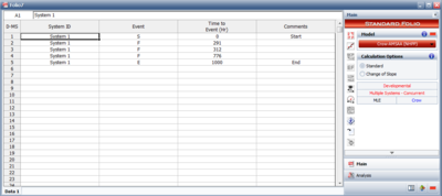
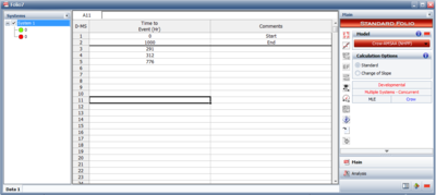
This data type is used for tests where a number of systems are tested, and the start and end of failure times are recorded. This data type assumes uniform time accumulation and that the systems are tested simultaneously. When a corrective action is implemented on a failed system, the fix is also applied to the non-failed systems. This results in all systems on test having the same configuration throughout the test. As an example, consider the data of two systems shown in the following figure. In this case, the folio is shown in Normal view.
System 1 begins testing at time equals 0 (with a start event, S). Note that when entering data within the Normal view, each system must be initiated with a start event. The failures encountered by System1 are corrected at 281, 312 and 776 (with failure events, F). Testing stops at 1000 hours (with an end event, E). System 2 begins testing at time equals 0 and failures are encountered and corrected at 40, 222 and 436. Testing stops at 500 hours.Systems with a start time greater than zero are shifted back to t = 0. This is the same as having a start time equal to zero and the converted end time is equal to the end time minus the start time. A start time greater than zero indicates that it is not known as to what events occurred at a time less than the start time. This may have been caused by the events during this period not being tracked and/or recorded properly.
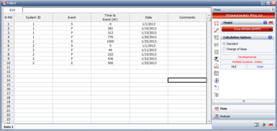
The next figure shows the folio and the same data set in the Advanced Systems view.
Multiple Systems with Dates
This is similar to Multiple Systems (Concurrent Operating Times) except that a date is now associated with each event. This assumes noncontinuous usage and the software computes equivalent (average) usage rates. The next figure shows an example of this in RGA.
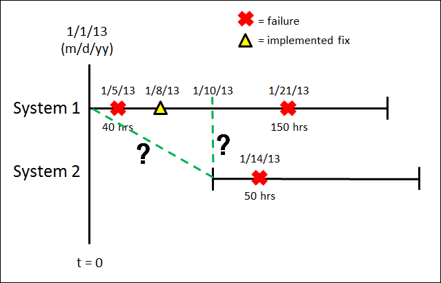
The question is when should Multiple Systems with Dates be used. In other words, when are dates important? Consider the picture below (not drawn to scale).
Two systems are placed in a reliability growth test. System 1 starts testing on January 1, 2013 and System 2 does not start testing until January 10, 2013. When testing begins on System 2, what is its configuration? Does the configuration of System 2 on January 10 match System 1 on January 10 (there was a fix implemented on System 1 on January 8) or does it match System 1's configuration on January 1? If the configuration of System 2 matches System 1 on January 1, then dates are not important and the previous data type, Multiple Systems (Concurrent Operating Times) can be used and the timeline for System 2 can be shifted to the left . However, if the configuration of System 2 matches System 1 on January 10 then dates are important and the Multiple Systems with Dates data type should be used. The goal is to sum up the accumulated hours across all systems with the same configuration. If System 2 on January 10 matches System 1 on January 10 then it would not be correct to shift System 2 to the left to t = 0. If this was done, the first failure on System 1 on January 5 would correspond to 80 hours, 40 hours for System 1 and 40 hours for System 2, on the equivalent system timeline. However, with dates this same failure now corresponds to 40 hours on the equivalent system timeline since System 2 is not operating yet.
For the failure on January 14 on System 2, the total test time on this date must also account for the test time accumulated on System 1. However, this is not an event on System 1 on January 14. Therefore, RGA uses linear interpolation to estimate the test time on System 1 on January 14.
Multiple Systems with Event Codes
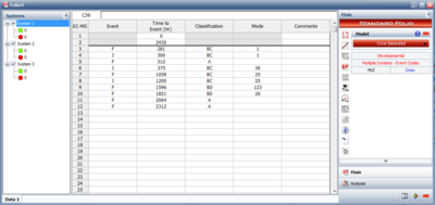
The Multiple Systems with Event Codes data type is used to analyze the failure data from a reliability growth test in which a number of systems are tested concurrently and the implemented fixes are tracked during the test phase. With this data type, all of the systems under test are assumed to have the same system hours at any given time. The next figure shows an example of this type of data.
Models for Time-to-Failure (Continuous) Data
The following models can be used to analyze time-to-failure (continuous) data sets. Models and examples using the different data types are discussed in later chapters.
- 1) Duane
Discrete Data
Discrete data are also referred to as success/failure or attribute data. These data sets consist of data from a test where a unit is tested with only two possible outcomes: success or failure. An example of this is a missile that gets fired once and it either succeeds or fails. The data types available for analyzing discrete data with the RGA software are:
- Sequential
- Sequential with Mode
- Grouped per Configuration
- Mixed Data
Sequential Data
For sequential data, an item is tested with only two possible outcomes: success or failure. This could be a one-shot item such as a missile or an entire system that either succeeds or fails. The item is then inspected after each trial and redesigned/repaired before the next trial. The following figure shows an example of this data type, where the row number in the data sheet represents the sequence of the trials. In this data set, trial #1 succeeded, trial #2 failed, and so on.
Sequential with Mode Data
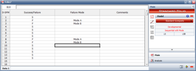
Often after failure analysis you know the reason for failure during a particular trial. If this is the case, the reason for each failure can also be used in the analysis. This data entry is identical to the sequential data with the exception that a failure code, mode or ID is added after each failure so that the analysis can take into account different failure modes. The next figure shows an example of this type of data.
Grouped per Configuration Data
This data type is used when multiple items, instead of a single item, are tested and the number of units that fail are recorded for each configuration. The row numbers that appear on the left side of the worksheet, as shown in the following figure, represent the unique configurations. For example, row 1 indicates configuration 1 in which 10 missiles were fired and 5 failed, row 2 indicates configuration 2 in which 8 missiles were fired and 3 failed, etc. The data can be cumulative or non-cumulative.
Mixed Data
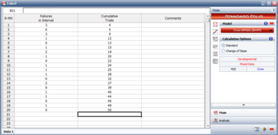
The mixed data type can have input data that is either for configurations in groups, individual trial by trial, or a mixed combination of individual trials and configurations of more than one trial. The following figure shows an example of this data type. For example the first row of this data sheet shows that 3 failures occurred in the first 4 trials, the second row shows that there were no failures in the next trial, while the third row shows that 3 failures occurred in the next 4 trials
Models for Discrete Data
The following models can be used to analyze discrete data. Models and examples using the different data types are discussed in later chapters.
- 1) Duane
- 4) Lloyd-Lipow
- 6) Logistic
Multi-Phase Data
Reliability data can be analyzed across multiple phases. This is useful when an overall reliability growth program is planned and involves multiple test phases.
(Multi-Phase) Failure Times Data
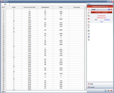
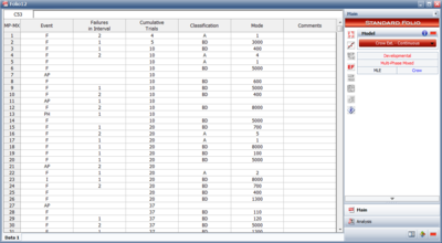
This data type can be used for tests that span multiple phases and the exact failure times are recorded. The figure below shows an example of multi-phase failure times data, where the different events signify failures (F), test phases (PH) or analysis points (AP).
(Multi-Phase) Grouped Failure Times Data
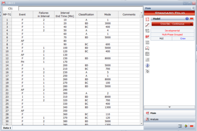
This data type can be used for tests that span multiple phases and the exact failure times are unknown. Only the number of failures within a time interval are recorded, as shown in the figure below.
(Multi-Phase) Mixed Data
This data type can be used for tests that span multiple phases and it allows for configuration in groups, individual trial by trial, or a mixed combination of individual trials and configurations of more than one trial. An example of this data type can be seen in the figure below.
Models for Multi-Phase Data
The Crow Extended - Continuous Evaluation model is used to analyze data across multiple phases.
Reliability Data
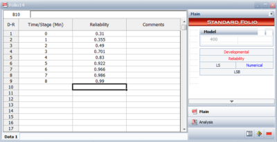
Reliability data consists of entering the reliability of the equipment at different times or stages. An example is shown in the figure below. In this case, the process is monitored at pre-defined time intervals and the reliability is recorded. The reliability can be computed by a simple ratio of the number of units still functioning vs. the number of units that entered the test stage or by using life data analysis and related methods (e.g., Weibull analysis).
Models for Reliability Data
The following models can be used to analyze reliability data sets. Models and examples using different data types are discussed in later chapters.
- 1) Lloyd-Lipow
- 3) Logistic
Fielded Systems
Fielded systems are systems that are used by customers in the field and for which failure information is not derived from an in-house test. This type of data is analogous to warranty data. The data types available for fielded systems data entry are:
- Repairable Systems
- Fleet
Repairable Systems
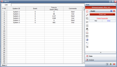
Repairable Systems data is identical in format to the Multiple Systems (Concurrent Operating Times) data. It also can be entered in the Normal or Advanced Systems view. The following figure illustrates a sample data set. In repairable systems, the purpose of the analysis is not to evaluate reliability growth but rather to obtain reliability estimates for the system, including expected number of failures, reliability at a given time, and so forth.
Models for Repairable Systems Data
The following models can be used to analyze repairable systems data. Models and examples using different data types are discussed in RGA Models for Repairable Systems Analysis.
- 1) Power Law
- 2) Crow Extended
Fleet Data
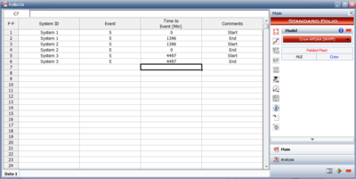
This data type is used to analyze the entire population (fleet). The data entry for this data type is similar to the data entry for repairable systems; however, the overall data analysis is again different. In repairable systems, the reliability of a single system can be tracked and quantified, whereas in a fleet analysis, data from the entire fleet as a whole is analyzed. The figure below presents an example of data entered for fleet analysis.
Models for Fleet Data
The following models can be used to analyze fleet data. Models and examples using different data types are discussed in later chapters.

