Warranty Data Analysis Times-to-Failure Format with Plot Example
New format available! This reference is now available in a new format that offers faster page load, improved display for calculations and images and more targeted search.
As of January 2024, this Reliawiki page will not continue to be updated. Please update all links and bookmarks to the latest references at Weibull examples and Weibull reference examples.
The warranty analysis folio includes different formats to accommodate several types of claims data. The Times-to-Failure format is the simplest format because it is similar to a Weibull++ standard folio, but with added functionality to generate forecasts.
Times-to-Failure Format Warranty Analysis
Assume that we have the following information for a given product.
| Number in State | State F or S | State End Time (Hr) |
| 2 | F | 100 |
| 3 | F | 125 |
| 5 | F | 175 |
| 1500 | S | 200 |
| Quantity In-Service | Time (Hr) |
| 500 | 200 |
| 400 | 300 |
| 100 | 500 |
Use the time-to-failure warranty analysis folio to analyze the data and generate a forecast for future returns.
Solution
Create a warranty analysis folio and select the times-to-failure format. Enter the data from the tables in the Data and Future Sales sheets, and then analyze the data using the 2P-Weibull distribution and RRX analysis method. The parameters are estimated to be beta = 3.199832 and eta=814.293442.
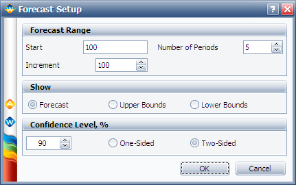
Click the Forecast icon on the control panel. In the Forecast Setup window, set the forecast to start on the 100th hour and set the number of forecast periods to 5. Set the increment (length of each period) to 100, as shown next.
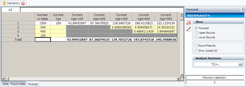
Click OK. A Forecast sheet will be created, with the following predicted future returns.
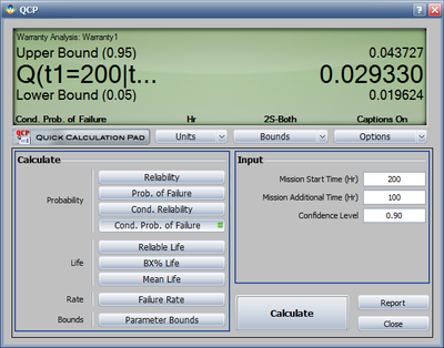
We will use the first row to explain how the forecast for each cell is calculated. For example, there are 1,500 units with a current age of 200 hours. The probability of failure in the next 100 hours can be calculated in the QCP, as follows.
Therefore, the predicted number of failures for the first 100 hours is:
- [math]\displaystyle{ 1500\times 0.02932968=43.99452\,\! }[/math]
This is identical to the result given in the Forecast sheet (shown in the 3rd cell in the first row) of the analysis. The bounds and the values in other cells can be calculated similarly.
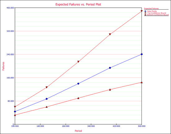
All the plots that are available for the standard folio are also available in the warranty analysis, such as the Probability plot, Reliability plot, etc. One additional plot in warranty analysis is the Expected Failures plot, which shows the expected number of failures over time. The following figure shows the Expected Failures plot of the example, with confidence bounds.


