Warranty Analysis Usage Format Example

New format available! This reference is now available in a new format that offers faster page load, improved display for calculations and images and more targeted search.

As of January 2024, this Reliawiki page will not continue to be updated. Please update all links and bookmarks to the latest references at Weibull examples and Weibull reference examples.

---

This example appears in the Life Data Analysis Reference book.

Warranty Analysis Usage Format Example

Suppose that an automotive manufacturer collects the warranty returns and sales data given in the following tables. Convert this information to life data and analyze it using the lognormal distribution.

Quality In-Service Data

Quantity In-Service	Date In-Service
9	Dec-09
13	Jan-10
15	Feb-10
20	Mar-10
15	Apr-10
25	May-10
19	Jun-10
16	Jul-10
20	Aug-10
19	Sep-10
25	Oct-10
30	Nov-10

Quality Return Data

Quantity Returned	Usage at Return Date	Return Date
1	9072	Dec-09
1	9743	Jan-10
1	6857	Feb-10
1	7651	Mar-10
1	5083	May-10
1	5990	May-10
1	7432	May-10
1	8739	May-10
1	3158	Jun-10
1	1136	Jul-10
1	4646	Aug-10
1	3965	Sep-10
1	3117	Oct-10
1	3250	Nov-10

Solution

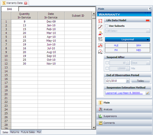
Create a warranty analysis folio and select the usage format. Enter the data from the tables in the Sales, Returns and Future Sales sheets. The warranty data were collected until 12/1/2010; therefore, on the control panel, set the End of Observation Period to that date. Set the failure distribution to Lognormal, as shown next.

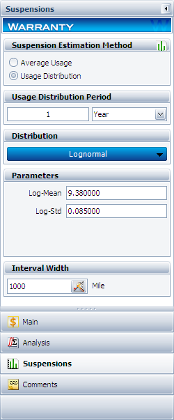
In this example, the manufacturer has been documenting the mileage accumulation per year for this type of product across the customer base in comparable regions for many years. The yearly usage has been determined to follow a lognormal distribution with [math]\displaystyle{ {{\mu }_{T\prime }}=9.38 }[/math] , [math]\displaystyle{ {{\sigma }_{T\prime }}=0.085 }[/math]. The Interval Width is defined to be 1000 miles. Enter the information about the usage distribution on the Usage page of the control panel, as shown next.

Click Calculate to analyze the data set. The parameters are estimated to be:

[math]\displaystyle{ \begin{align} & {{\mu }_{T\prime }}= & 10.528098 \\ & {{\sigma }_{T\prime }}= & 1.135150 \end{align} }[/math]

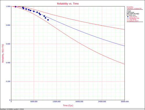
The reliability plot (with mileage being the random variable driving reliability), along with the 90% confidence bounds on reliability, is shown next.