Example: Weibull Degradation Crack Propagation (Point Estimation)
Five turbine blades were tested for crack propagation. The test units are cyclically stressed and inspected every 100,000 cycles for crack length. Failure is defined as a crack of length 30mm or greater.
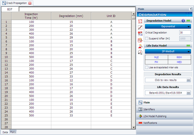
Following is a table of the test results:
Using degradation analysis with an exponential model for the extrapolation, determine the B10 life for the blades.
Solution
The first step is to solve the equation [math]\displaystyle{ y=b\cdot {{e}^{a\cdot x}} }[/math] for [math]\displaystyle{ a }[/math] and [math]\displaystyle{ b }[/math] for each of the test units. Using regression analysis, these values for each of the test units are:
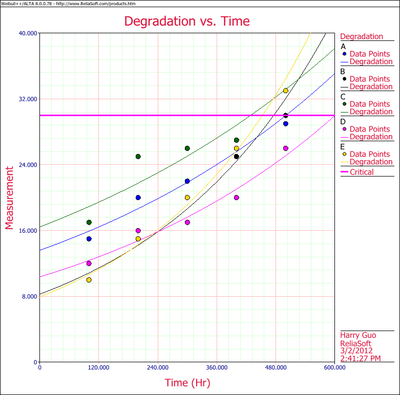
These results are shown graphically in the next figure.
[math]\displaystyle{ }[/math]
These values can now be substituted into the underlying exponential model, solved for [math]\displaystyle{ x }[/math] or:
Using the values of [math]\displaystyle{ a }[/math] and [math]\displaystyle{ b }[/math] , with [math]\displaystyle{ y=30 }[/math] , the resulting time at which the crack length reaches 30mm is then found for each sample:
These times-to-failure can now be analyzed in the conventional manner. Assuming a two-parameter Weibull distribution and using the MLE estimation method, the distribution parameters are calculated as [math]\displaystyle{ \beta =8.055 }[/math] and [math]\displaystyle{ \eta =519,555. }[/math] Using these values, the B10 life is calculated to be 392,918 cycles. The degradation analysis tool in Weibull++ performs this type of analysis for you. The following figure shows the data as entered in Weibull++ for this analysis.
[math]\displaystyle{ }[/math]


