Competing Failure Modes Example

Competing Failures with Two Failure Modes Example

From Meeker & Escobar [27], the following table gives failure times for an electric component that has two failure modes.

One failure mode is due to random voltage spikes which cause failure by overloading the system (denoted as a [math]\displaystyle{ V }[/math] in the table). The other failure mode is due to wear-out failures which usually happen only after the system has run for many cycles (this failure mode is denoted as a [math]\displaystyle{ W }[/math] in the table).

Considering that these are competing failure modes, determine the overall reliability for the component at 100,000 cycles.

[math]\displaystyle{ \begin{matrix} Number & Failure & Failure & Number & Failure & Failure \\ in State & Time* & Mode & in State & Time* & Mode \\ \text{1} & \text{2} & \text{V} & \text{1} & \text{147} & \text{W} \\ \text{1} & \text{10} & \text{V} & \text{1} & \text{173} & \text{V} \\ \text{1} & \text{13} & \text{V} & \text{1} & \text{181} & \text{W} \\ \text{2} & \text{23} & \text{V} & \text{1} & \text{212} & \text{W} \\ \text{1} & \text{28} & \text{V} & \text{1} & \text{245} & \text{W} \\ \text{1} & \text{30} & \text{V} & \text{1} & \text{247} & \text{V} \\ \text{1} & \text{65} & \text{V} & \text{1} & \text{261} & \text{V} \\ \text{1} & \text{80} & \text{V} & \text{1} & \text{266} & \text{W} \\ \text{1} & \text{88} & \text{V} & \text{1} & \text{275} & \text{W} \\ \text{1} & \text{106} & \text{V} & \text{1} & \text{293} & \text{W} \\ \text{1} & \text{143} & \text{V} & \text{8} & \text{300} & \text{suspended} \\ \end{matrix} }[/math]

• Failure times given are in thousands of cycles.

Solution

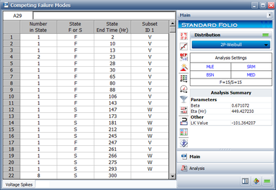
We will begin by performing a Weibull analysis of the voltage spike ( [math]\displaystyle{ V }[/math] ) failure mode. In order to do this, we must consider all of the failures for the wear-out mode to be suspensions. The input data for the analysis are shown next:

Analyzing this data set using the maximum likelihood method (recommended due to the number of suspensions in the data) and assuming a Weibull distribution, we obtain the parameters [math]\displaystyle{ {{\beta }_{V}}=0.6711 }[/math] and [math]\displaystyle{ {{\eta }_{V}}=449.4 }[/math] . The reliability for this failure mode at [math]\displaystyle{ t=100 }[/math] is [math]\displaystyle{ {{R}_{V}}(100)=0.694 }[/math] .

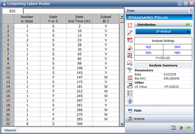
We follow an identical procedure for the wear-out failure mode, counting only the [math]\displaystyle{ W }[/math] entries as failures and assuming the [math]\displaystyle{ V }[/math] entries are suspensions. This is shown next.

Once again, analyzing with a Weibull distribution with maximum likelihood estimators, we obtain the parameters [math]\displaystyle{ {{\beta }_{W}}=4.337 }[/math] and [math]\displaystyle{ {{\eta }_{W}}=340.4 }[/math] . The reliability for this failure mode at [math]\displaystyle{ t=100 }[/math] is [math]\displaystyle{ {{R}_{W}}(100)=0.995 }[/math] .

We can now use the system Reliability Equation to determine the overall system reliability at 100,000 cycles:

[math]\displaystyle{ \begin{align} & {{R}_{sys}}(100)= {{R}_{V}}(100)\cdot {{R}_{W}}(100) \\ & = 0.694\cdot 0.995 \\ & = 0.69053 \end{align} }[/math]

Or the reliability of the unit (or system) under both modes is [math]\displaystyle{ {{R}_{sys}}(100)=69.053%. }[/math]

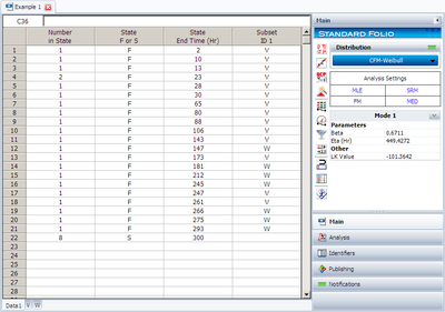
Note that Weibull++ can perform this analysis for you automatically. To accomplish this, the data would be entered in a single data sheet and competing failure modes chosen as the analysis method. This is shown in the next graphic.