Template:Example: Wei-Bayesian Log-normal Prior

Weibull-Bayesian with Lognormal Prior Example

A manufacturer has tested prototypes of a modified product. The test was terminated at 2000 hours, with only two failures observed from a sample size of eighteen.

Number of State	State of F or S	State End Time
1	F	1180
1	F	1842
16	S	2000

Because of the lack of failure data in the prototype testing, the manufacturer decided to use information gathered from prior tests on this product to increase the confidence in the results of the prototype testing. This decision was made because failure analysis indicated that the failure mode of these two failures is the same as the one observed in previous tests. In other words, it is expected that the shape of the distribution hasn't changed, but hopefully the scale has, indicating longer life. The two-parameter Weibull distribution have been used to model all prior tests results. The list of the estimated β parameter is as follows:

Betas Obtained for Similar Mode
1.7
2.1
2.4
3.1
3.5

Solution

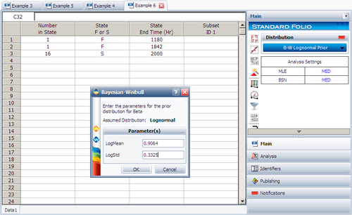
First, in order to fit the data to a Weibull-Bayesian model, a prior distribution for β needs to be determined. Based on the prior tests' β values, the prior distribution for β was found to be a lognormal distribution with μ = 0.9064, σ = 0.3325 (obtained by entering the β values into a Weibull++ Standard Folio and analyzing it based on the RRX analysis method.)

the test data is entered into a Standard Folio, the B-W Lognormal Prior is selected under Distribution and the β prior distribution is entered after clicking the Calculate button.

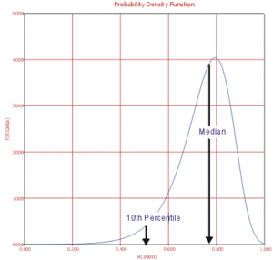
Suppose that the reliability at 3000hr is the metric of interest in this example. This reliability can be obtained using the equation for median reliability, resulting in the median value of the posterior of the reliability at 3000hr. Using the QCP, this value is calculated to be 76.97%. ( By default Weibull++ returns the median values of the posterior distribution. )

The posterior [math]\displaystyle{ pdf }[/math] of the reliability function at 3000hrs can be obtained using the equation at the begining of this section. In Figure 6-10 the posterior [math]\displaystyle{ pdf }[/math] of the reliability at 3000hrs is plotted, with the corresponding median value as well as the 10th percentile value shown. The 10th percentile constitutes the 90 Lower 1-Sided bound on the reliability at 3000hrs, which is calculated to be 50.77%.

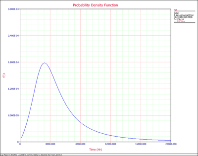
Notice that the [math]\displaystyle{ pdf }[/math] plotted in Fig. 6-10 is of the reliability at 3000hrs, and not the [math]\displaystyle{ pdf }[/math] of the times-to-failure data. The [math]\displaystyle{ pdf }[/math] of the times-to-failure data can be obtained using the equation at the begining of this section and plotted using Weibull++, as shown next:

The material on this page is copyrighted.

©1992-2012. ReliaSoft Corporation. ALL RIGHTS RESERVED.