Template:Failure modes configurations

Failure Modes Configurations

Series Configuration

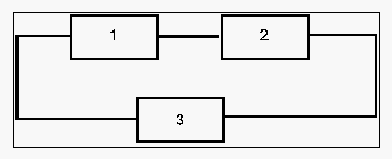
The basic competing failure modes configuration, which has already been discussed, is a series configuration. In a series configuration, the occurrence of any failure mode results in failure for the product.

The equation that describes series configuration is:

[math]\displaystyle{ R(t)={{R}_{1}}(t)\cdot {{R}_{2}}(t)\cdot ...\cdot {{R}_{n}}(t) }[/math]

where [math]\displaystyle{ n }[/math] is the total number of failure modes considered.

Parallel

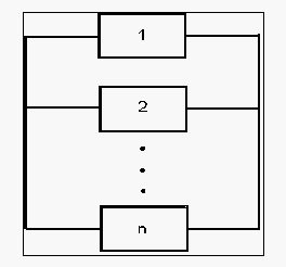
In a simple parallel configuration, at least one of the failure modes must not occur for the product to continue operation.

[math]\displaystyle{ }[/math]

The equation that describes parallel configuration is:

[math]\displaystyle{ R(t)=1-\underset{i=1}{\overset{n}{\mathop \prod }}\,(1-{{R}_{i}}(t)) }[/math]

where [math]\displaystyle{ n }[/math] is the total number of failure modes considered.

Combination of Series and Parallel

While many smaller products can be accurately represented by either a simple series or parallel configuration, there may be larger products that involve both series and parallel configurations in the overall model of the product. Such products can be analyzed by calculating the reliabilities for the individual series and parallel sections and then combining them in the appropriate manner.

[math]\displaystyle{ }[/math]

k-out-of-n Parallel Configuration=

The k-out-of-n configuration is a special case of parallel redundancy. This type of configuration requires that at least [math]\displaystyle{ k }[/math] failure modes do not happen out of the total [math]\displaystyle{ n }[/math] parallel failure modes for the product to succeed. The simplest case of a k-out-of-n configuration is when the failure modes are independent and identical and have the same failure distribution and uncertainties about the parameters (in other words they are derived from the same test data). In this case, the reliability of the product with such a configuration can be evaluated using the binomial distribution, or:

[math]\displaystyle{ R(t)=\overset{n}{\mathop{\underset{r=k}{\mathop{\underset{}{\overset{}{\mathop \sum }}\,}}\,}}\,\left( \underset{k}{\mathop{\overset{n}{\mathop{{}}}\,}}\, \right){{R}^{r}}(t){{(1-R(t))}^{n-r}} }[/math]

In the case where the k-out-of-n failure modes are not identical, other approaches for calculating the reliability must be used (e.g. the event space method). Discussion of these is beyond the scope of this reference. Interested readers can consult ReliaSoft's System Reliability Reference.

Complex Systems

In many cases, it is not easy to recognize which components are in series and which are in parallel in a complex system.

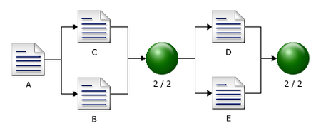
The previous configuration cannot be broken down into a group of series and parallel configurations. This is primarily due to the fact that failure mode C has two paths leading away from it, whereas B and D have only one. Several methods exist for obtaining the reliability of a complex configuration including the decomposition method, the event space method and the path-tracing method. Discussion of these is beyond the scope of this reference. Interested readers can consult ReliaSoft's System Reliability Reference.

Example 2:

Assume that a product has five independent failure modes: A, B, C, D and E. Furthermore, assume that failure of the product will occur if mode A occurs, modes B and C occur simultaneously or if modes D and E occur simultaneously. The objective is to estimate the reliability of the product at 100 hours, with 90% two-sided confidence bounds.

The product is tested to failure, and the failure times due to each mode are recorded in the following table.

TTF for A	TTF for B	TTF for C	TTF for D	TTF for E
276	23	499	467	67
320	36	545	540	72
323	57	661	716	81
558	89	738	737	108
674	99	987	761	110
829	154	1165	1093	127
878	200	1337	1283	148

Solution

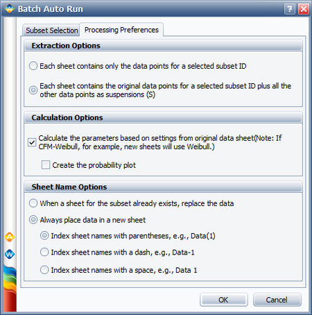
The reliability block diagram (RBD) approach can be used to analyze the reliability of the product. But before creating a diagram, the data sets of the failure modes need to be segregated so that each mode can be represented by a single block in the diagram. Recall that when you analyze a particular mode, the failure times for all other competing modes are considered to be suspensions. This captures the fact that those units operated for a period of time without experiencing the failure mode of interest before they were removed from observation when they failed due to another mode. We can easily perform this step via Weibull++'s Batch Auto Run utility. To do this, enter the data from the table into a single data sheet. Choose the 2P-Weibull distribution and the MLE analysis method, and then click the Batch Auto Run icon on the control panel. When prompted to select the subset IDs, select them all. Click the Processing Preferences tab. In the Extraction Options area, select the second option, as shown next.

This will extract the data sets that are required for the analysis. Select the check box in the Calculation Options area and click OK. The data sets are extracted into separate data sheets in the folio and automatically calculated.

Next, create a diagram by choosing Insert > Tools > Diagram. Add blocks by right-clicking the diagram and choosing Add Block on the shortcut menu. When prompted to select the data sheet of the failure mode that the block will represent, select the data sheet for mode A. Use the same approach to add the blocks that will represent failure modes B, C , D and E. Add a connector by right-clicking the diagram sheet and choosing Connect Blocks, and then connect the blocks in an appropriate configuration to describe the relationships between the failure modes. To insert a node, which acts as a switch that the diagram paths move through, right-click the diagram and choose Add Node. Specify the number of required paths in the node by double-clicking the node and entering the appropriate number (use 2 in both nodes).

The following figure shows the completed diagram.

Click Analyze to analyze the diagram, and then use the Quick Calculation Pad (QCP) to estimate the reliability. The estimated R(100 hours) and the 90% two-sided confidence bounds are:

[math]\displaystyle{ \begin{matrix} {{{\hat{R}}}_{U}}(100)=0.895940 \\ \hat{R}(100)=0.824397 \\ {{{\hat{R}}}_{L}}(100)=0.719090 \\ \end{matrix}\,\! }[/math]