Template:Ipl lognormal

IPL-Lognormal

The pdf for the Inverse Power Law relationship and the lognormal distribution is given next.

The pdf of the lognormal distribution is given by:

[math]\displaystyle{ f(T)=\frac{1}{T\text{ }{{\sigma }_{{{T}'}}}\sqrt{2\pi }}{{e}^{-\tfrac{1}{2}{{\left( \tfrac{{T}'-\overline{{{T}'}}}{{{\sigma }_{{{T}'}}}} \right)}^{2}}}} }[/math]

where:

[math]\displaystyle{ T'=ln(T) }[/math].

and:

[math]\displaystyle{ T }[/math] = times-to-failure.

[math]\displaystyle{ \overline{T}' }[/math] = mean of the natural logarithms of the times-to-failure.

[math]\displaystyle{ \sigma_{T'} }[/math] = standard deviation of the natural logarithms of the times-to-failure.

The median of the lognormal distribution is given by:

[math]\displaystyle{ \breve{T}=e^{\overline{T}'} }[/math]

The IPL-lognormal model pdf can be obtained first by setting [math]\displaystyle{ \breve{T}=L(V) }[/math] in the lognormal [math]\displaystyle{ pdf }[/math]. Therefore:

[math]\displaystyle{ \breve{T}=L(V)=\frac{1}{K \cdot V^n} }[/math]

or:

[math]\displaystyle{ e^{\overline{T'}}=\frac{1}{K \cdot V^n} }[/math]

Thus:

[math]\displaystyle{ \overline{T}'=-ln(K)-n ln(V) }[/math]

So the IPL-lognormal model [math]\displaystyle{ pdf }[/math] is:

[math]\displaystyle{ f(T,V)=\frac{1}{T\text{ }{{\sigma }_{{{T}'}}}\sqrt{2\pi }}{{e}^{-\tfrac{1}{2}{{\left( \tfrac{{T}'+ln(K)+n ln(V)}{{{\sigma }_{{{T}'}}}} \right)}^{2}}}} }[/math]

The Mean

The mean life of the IPL-lognormal model (mean of the times-to-failure), [math]\displaystyle{ \bar{T} }[/math] , is given by:

[math]\displaystyle{ \bar{T}=\ {{e}^{\bar{{T}'}+\tfrac{1}{2}\sigma _{{{T}'}}^{2}}}= {{e}^{{-ln(K)-nln(V)}+\tfrac{1}{2}\sigma _{{{T}'}}^{2}}} }[/math]

The mean of the natural logarithms of the times-to-failure, [math]\displaystyle{ {{\bar{T}}^{^{\prime }}} }[/math] , in terms of [math]\displaystyle{ \bar{T} }[/math] and [math]\displaystyle{ {{\sigma }_{T}} }[/math] is given by:

[math]\displaystyle{ {{\bar{T}}^{\prime }}=\ln \left( {\bar{T}} \right)-\frac{1}{2}\ln \left( \frac{\sigma _{T}^{2}}{{{{\bar{T}}}^{2}}}+1 \right) }[/math]

The Standard Deviation

The standard deviation of the IPL-lognormal model (standard deviation of the times-to-failure), [math]\displaystyle{ {{\sigma }_{T}} }[/math] , is given by:

[math]\displaystyle{ \begin{align} {{\sigma }_{T}}= & \sqrt{\left( {{e}^{2\bar{{T}'}+\sigma _{{{T}'}}^{2}}} \right)\,\left( {{e}^{\sigma _{{{T}'}}^{2}}}-1 \right)} = \sqrt{\left( {{e}^{2\left( -\ln (K)-n\ln (V) \right)+\sigma _{{{T}'}}^{2}}} \right)\,\left( {{e}^{\sigma _{{{T}'}}^{2}}}-1 \right)} \end{align} }[/math]

The standard deviation of the natural logarithms of the times-to-failure, [math]\displaystyle{ {{\sigma }_{{{T}'}}} }[/math] , in terms of [math]\displaystyle{ \bar{T} }[/math] and [math]\displaystyle{ {{\sigma }_{T}} }[/math] is given by:

[math]\displaystyle{ {{\sigma }_{{{T}'}}}=\sqrt{\ln \left( \frac{\sigma _{T}^{2}}{{{{\bar{T}}}^{2}}}+1 \right)} }[/math]

The Mode

The mode of the IPL-lognormal model is given by:

IPL-Lognormal Reliability

The reliability for a mission of time T, starting at age 0, for the IPL-lognormal model is determined by:

or:

Reliable Life

The reliable life, or the mission duration for a desired reliability goal, tR is estimated by first solving the reliability equation with respect to time, as follows:

where:

and:

Since = ln(T) the reliable life, tR, is given by:

Lognormal Failure Rate

The lognormal failure rate is given by:

Parameter Estimation

Maximum Likelihood Estimation Method

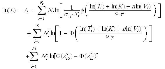
The complete IPL-lognormal log-likelihood function is:

where:

and:

• Fe is the number of groups of exact times-to-failure data points.

• Ni is the number of times-to-failure data points in the ith time-to-failure data group.

• [math]\displaystyle{ s_{T'} }[/math] is the standard deviation of the natural logarithm of the times-to-failure (unknown, the first of three parameters to be estimated).

• [math]\displaystyle{ K }[/math] is the IPL parameter (unknown, the second of three parameters to be estimated).

• [math]\displaystyle{ n }[/math] is the second IPL parameter (unknown, the third of three parameters to be estimated).

• [math]\displaystyle{ Vi }[/math] is the stress level of the ith group.

• [math]\displaystyle{ Ti }[/math] is the exact failure time of the ith group.

• [math]\displaystyle{ S }[/math] is the number of groups of suspension data points.

• [math]\displaystyle{ N'_i }[/math] is the number of suspensions in the ith group of suspension data points.

• [math]\displaystyle{ T^{'}_{i} }[/math] is the running time of the ith suspension data group.

• [math]\displaystyle{ FI }[/math] is the number of interval data groups.

• is the number of intervals in the ith group of data intervals.

• is the beginning of the ith interval.

• is the ending of the ith interval.

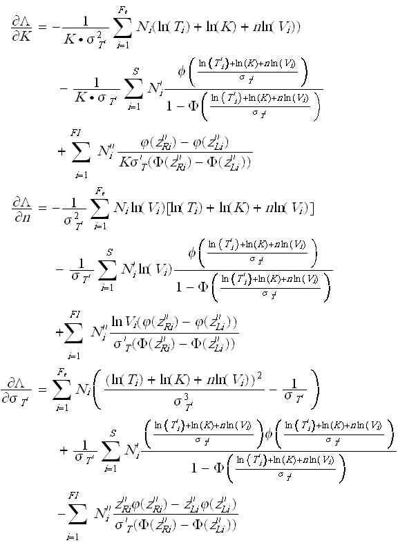
The solution (parameter estimates) will be found by solving for , , so that = 0, = 0 and = 0:

and: