Template:Ipl ex rel function
IPL-Exponential Reliability Function
The IPL-exponential reliability function is given by:
This function is the complement of the IPL-exponential cumulative distribution function:
- or:
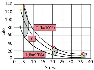
The inverse power law (IPL) model (or relationship) is commonly used for non-thermal accelerated stresses and is given by:
where:
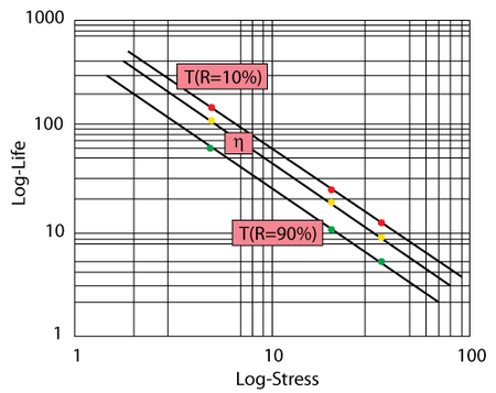
The inverse power law appears as a straight line when plotted on a log-log paper. The equation of the line is given by:
Plotting methods are widely used in estimating the parameters of the inverse power law relationship since obtaining
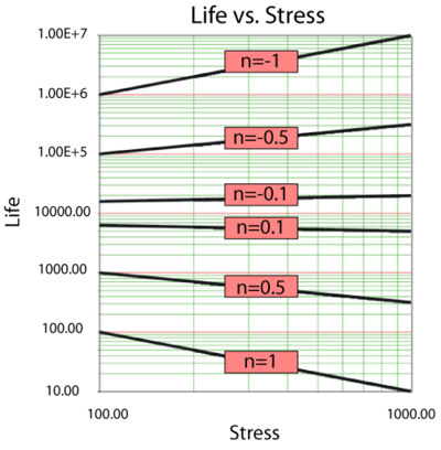
A Look at the Parameter n
The parameter
Acceleration Factor
For the IPL relationship the acceleration factor is given by:
where:
IPL-Exponential
The IPL-exponential model can be derived by setting
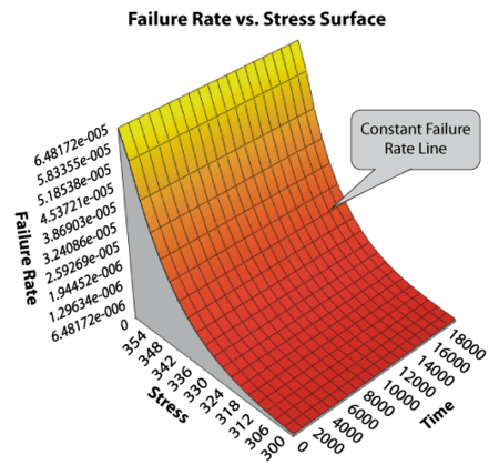
Note that this is a 2-parameter model. The failure rate (the parameter of the exponential distribution) of the model is simply
IPL-Exponential Statistical Properties Summary
Mean or MTTF
The mean,
Note that the MTTF is a function of stress only and is simply equal to the IPL relationship (which is the original assumption), when using the exponential distribution.
Median
The median,
Mode
The mode,
Standard Deviation
The standard deviation,
IPL-Exponential Reliability Function
The IPL-exponential reliability function is given by:
This function is the complement of the IPL-exponential cumulative distribution function:
or:
Conditional Reliability
The conditional reliability function for the IPL-exponential model is given by:
Reliable Life
For the IPL-exponential model, the reliable life or the mission duration for a desired reliability goal,
or:
Parameter Estimation
Maximum Likelihood Parameter Estimation
Substituting the inverse power law relationship into the exponential log-likelihood equation yields:
where:
and:
The solution (parameter estimates) will be found by solving for the parameters
IPL-Weibull
The IPL-Weibull model can be derived by setting
This is a three parameter model. Therefore it is more flexible but it also requires more laborious techniques for parameter estimation. The IPL-Weibull model yields the IPL-exponential model for
IPL-Weibull Statistical Properties Summary
Mean or MTTF
The mean,
where
Median
The median,
Mode
The mode,
Standard Deviation
The standard deviation,
IPL-Weibull Reliability Function
The IPL-Weibull reliability function is given by:
Conditional Reliability Function
The IPL-Weibull conditional reliability function at a specified stress level is given by:
- or:
Reliable Life
For the IPL-Weibull model, the reliable life,
IPL-Weibull Failure Rate Function
The IPL-Weibull failure rate function,
Parameter Estimation
Maximum Likelihood Estimation Method
Substituting the inverse power law relationship into the Weibull log-likelihood function yields:
where:
and:
The solution (parameter estimates) will be found by solving for
IPL-Weibull Example
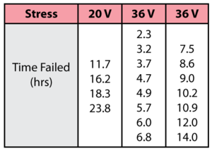
Consider the following times-to-failure data at two different stress levels.
The data set was analyzed jointly in an ALTA standard folio using the IPL-Weibull model, with a complete MLE solution over the entire data set. The analysis yields:
IPL-Lognormal
The pdf for the Inverse Power Law relationship and the lognormal distribution is given next.
The pdf of the lognormal distribution is given by:
where:
and:
The median of the lognormal distribution is given by:
The IPL-lognormal model pdf can be obtained first by setting
or:
Thus:
So the IPL-lognormal model pdf is:
IPL-Lognormal Statistical Properties Summary
The Mean
The mean life of the IPL-lognormal model (mean of the times-to-failure),
The mean of the natural logarithms of the times-to-failure,
The Standard Deviation
The standard deviation of the IPL-lognormal model (standard deviation of the times-to-failure),
The standard deviation of the natural logarithms of the times-to-failure,
The Mode
The mode of the IPL-lognormal model is given by:
IPL-Lognormal Reliability
The reliability for a mission of time T, starting at age 0, for the IPL-lognormal model is determined by:
or:
Reliable Life
The reliable life, or the mission duration for a desired reliability goal,
where:
and:
Since
Lognormal Failure Rate
The lognormal failure rate is given by:
Parameter Estimation
Maximum Likelihood Estimation Method
The complete IPL-lognormal log-likelihood function is:
where:
and:
The solution (parameter estimates) will be found by solving for
and:
IPL and the Coffin-Manson Relationship
In accelerated life testing analysis, thermal cycling is commonly treated as a low-cycle fatigue problem, using the inverse power law relationship. Coffin and Manson suggested that the number of cycles-to-failure of a metal subjected to thermal cycling is given by Nelson [28]:
where:
This relationship is basically the inverse power law relationship, where the stress
Example
In this example the use of the Coffin-Manson relationship will be illustrated. This is a very simple example which can be repeated at any time. The reader is encouraged to perform this test.
Product: ACME Paper Clip Model 4456
Reliability Target: 99% at a 90% confidence after 30 cycles of 45º
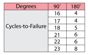
After consulting with our paper-clip engineers, the acceleration stress was determined to be the angle to which the clips are bent. Two bend stresses of 90º and 180º were used. A sample of six paper clips was tested to failure at both 90º and 180º bends with the following data obtained.
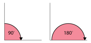
The test was performed as shown in the next figures (a side-view of the paper-clip is shown).
Using the IPL-lognormal model, determine whether the reliability target was met.
Solution
By using the IPL relationship to analyze the data, we are actually using a constant stress model to analyze a cycling process. Caution must be exercised when performing the test. The rate of change in the angle must be constant and equal for both the 90º and 180º bends and constant and equal to the rate of change in the angle for the use life of 45º bend. Rate effects are influencing the life of the paper clip. By keeping the rate constant and equal at all stress levels, we can then eliminate these rate effects from our analysis. Otherwise the analysis will not be valid.
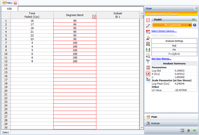
The data were entered and analyzed using ReliaSoft's ALTA.
The parameters of the IPL-lognormal model were estimated to be:
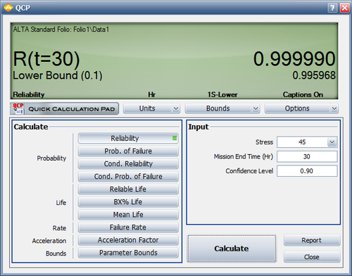
Using the QCP, the 90% lower 1-sided confidence bound on reliability after 30 cycles for a 45º bend was estimated to be
This meets the target reliability of 99%.
IPL Confidence Bounds
Approximate Confidence Bounds on IPL-Exponential
Confidence Bounds on the Mean Life
From the inverse power law relationship the mean life for the exponential distribution is given by setting
where
If
or:
The variances and covariance of
Confidence Bounds on Reliability
The bounds on reliability at a given time,
Confidence Bounds on Time
The bounds on time (ML estimate of time) for a given reliability are estimated by first solving the reliability function with respect to time:
The corresponding confidence bounds are estimated from:
Approximate Confidence Bounds on IPL-Weibull
Bounds on the Parameters
Using the same approach as previously discussed (
and:
The variances and covariances of
Confidence Bounds on Reliability
The reliability function (ML estimate) for the IPL-Weibull model is given by:
or:
Setting:
or:
The reliability function now becomes:
The next step is to find the upper and lower bounds on
where:
or:
The upper and lower bounds on reliability are:
Confidence Bounds on Time
The bounds on time for a given reliability (ML estimate of time) are estimated by first solving the reliability function with respect to time:
or:
where
where:
or:
The upper and lower bounds on time are then found by:
Approximate Confidence Bounds on IPL-Lognormal
Bounds on the Parameters
Since the standard deviation,
and:
The lower and upper bounds on
The variances and covariances of
where:
Bounds on Reliability
The reliability of the lognormal distribution is:
Let
For
The bounds on
where:
or:
The upper and lower bounds on reliability are:
Confidence Bounds on Time
The bounds around time, for a given lognormal percentile (unreliability), are estimated by first solving the reliability equation with respect to time, as follows:
where:
and:
The next step is to calculate the variance of
or:
The upper and lower bounds are then found by:
Solving for

