Template:Mixed weibull, other uses
Mixed Weibull, Other Uses
Reliability Bathtub Curves
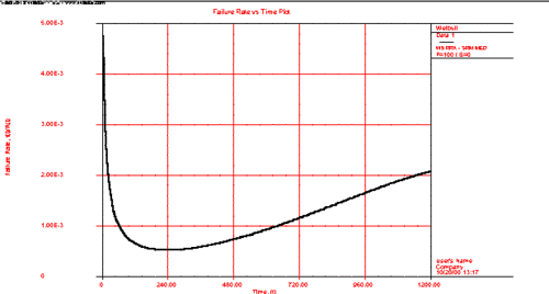
A reliability bathtub curve is nothing more than the graph of the failure rate versus time, over the life of the product. In general, the life stages of the product consist of early, chance and wear-out. Weibull++ allows you to plot this by simply selecting the failure rate plot, as shown next.
Determination of the Burn-in Period
If the failure rate goal is known, then the burn-in period can be found from the failure rate plot by drawing a horizontal line at the failure rate goal level and then finding the intersection with the failure rate curve. Next, drop vertically at the intersection, and read off the burn-in time from the time axis. This burn-in time helps insure that the population will have a failure rate that is at least equal to or lower than the goal after the burn-in period. The same could also be obtained using the Function Wizard and generating different failure rates based on time increments. Using these generated times and the corresponding failure rates, one can decide on the optimum burn-in time versus the corresponding desired failure rate.
We will illustrate the mixed Weibull analysis using a Monte Carlo generated set of data. To repeat this example, generate data from a 2-parameter Weibull distribution using the Weibull++ Monte Carlo utility. The following figures illustrate the required steps, inputs and results.
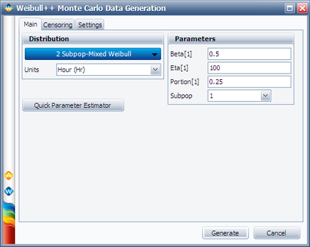
In the Monte Carlo window, enter the values and select the options shown below for subpopulation 1.
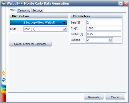
Switch to subpopulation 2 and make the selection shown below. Click Generate.
The simulation settings are:
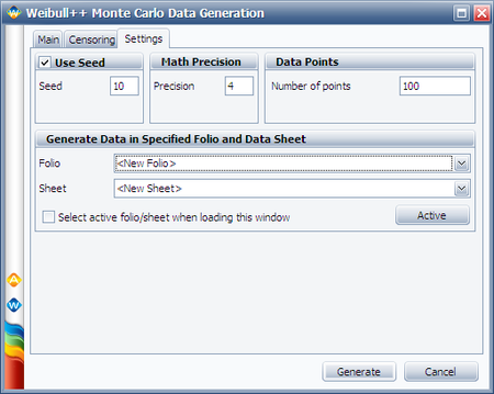
After the data set has been generated, choose the 2 Subpop-Mixed Weibull distribution. Click Calculate.
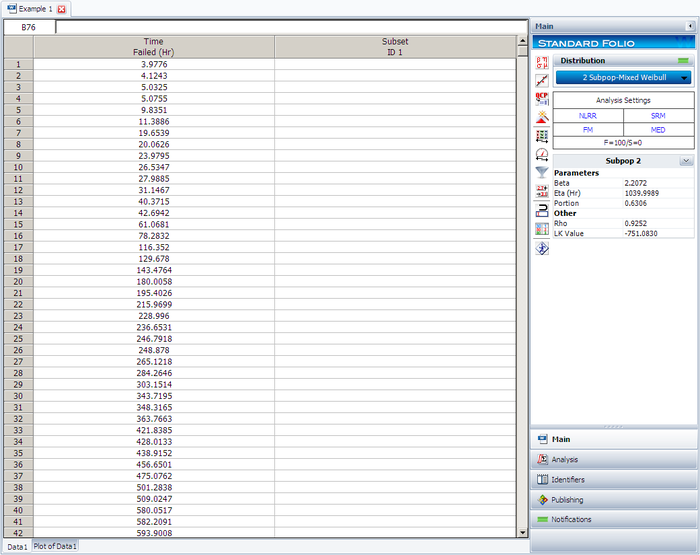
The results for subpopulation 1 are shown next. (Note that your results could be different due to the randomness of the simulation.)

The results for subpopulation 2 are shown next. (Note that your results could be different due to the randomness of the simulation.)
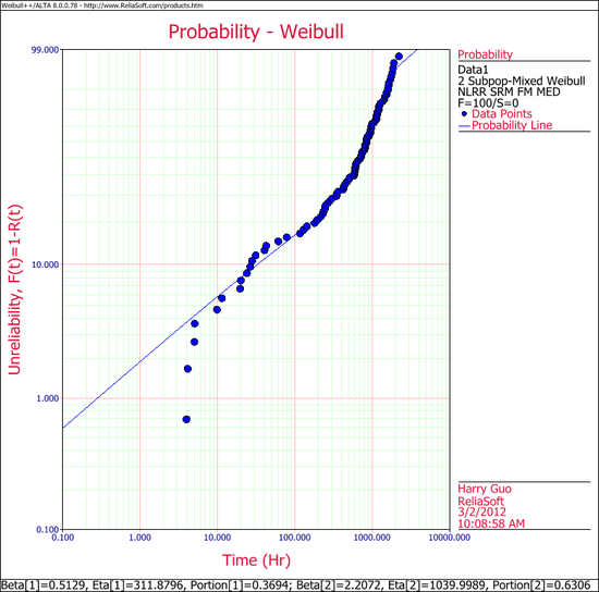
The Weibull probability plot for this data is shown next. (Note that your results could be different due to the randomness of the simulation.)
