Examples
Non-parametric analysis allows the user to analyze data without assuming an underlying distribution. This can have certain advantages as well as disadvantages. The ability to analyze data without assuming an underlying life distribution avoids the potentially large errors brought about by making incorrect assumptions about the distribution. On the other hand, the confidence bounds associated with non-parametric analysis are usually much wider than those calculated via parametric analysis, and predictions outside the range of the observations are not possible. Some practitioners recommend that any set of life data should first be subjected to a non-parametric analysis before moving on to the assumption of an underlying distribution.
There are several methods for conducting a non-parametric analysis. In Weibull++, this includes the Kaplan-Meier, actuarial-simple and actuarial-standard methods. A method for attaching confidence bounds to the results of these non-parametric analysis techniques can also be developed. The basis of non-parametric life data analysis is the empirical cdf function, which is given by:
- [math]\displaystyle{ \widehat{F}(t)=\frac{observations\le t}{n}\,\! }[/math]
Note that this is similar to the Benard's approximation of the median ranks, as discussed in the Parameter Estimation chapter. The following non-parametric analysis methods are essentially variations of this concept.
Kaplan-Meier Estimator
The Kaplan-Meier estimator, also known as the product limit estimator, can be used to calculate values for non-parametric reliability for data sets with multiple failures and suspensions. The equation of the estimator is given by:
- [math]\displaystyle{ \widehat{R}({{t}_{i}})=\underset{j=1}{\overset{i}{\mathop \prod }}\,\frac{{{n}_{j}}-{{r}_{j}}}{{{n}_{j}}},\text{ }i=1,...,m\,\! }[/math]
where:
- [math]\displaystyle{ \begin{align} & m= \text{the total number of data points} \\ & n= \text{the total number of units} \end{align}\,\! }[/math]
The variable [math]\displaystyle{ {{n}_{i}}\,\! }[/math] is defined by:
- [math]\displaystyle{ {{n}_{i}}=n-\underset{j=0}{\overset{i-1}{\mathop \sum }}\,{{s}_{j}}-\underset{j=0}{\overset{i-1}{\mathop \sum }}\,{{r}_{j,}}\text{ }i=1,...,m\,\! }[/math]
where:
- [math]\displaystyle{ \begin{align} & {{r}_{j}}= \text{the number of failures in the }{{j}^{th}}\text{ data group} \\ & {{s}_{j}}= \text{the number of suspensions in the }{{j}^{th}}\text{ data group} \end{align}\,\! }[/math]
Note that the reliability estimate is only calculated for times at which one or more failures occurred. For the sake of calculating the value of [math]\displaystyle{ {{n}_{j}}\,\! }[/math] at time values that have failures and suspensions, it is assumed that the suspensions occur slightly after the failures, so that the suspended units are considered to be operating and included in the count of [math]\displaystyle{ {{n}_{j}}\,\! }[/math].
Kaplan-Meier Example
A group of 20 units are put on a life test with the following results.
Use the Kaplan-Meier estimator to determine the reliability estimates for each failure time.
Solution
Using the data and the reliability equation of the Kaplan-Meier estimator, the following table can be constructed:
As can be determined from the preceding table, the reliability estimates for the failure times are:
Actuarial-Simple Method
The actuarial-simple method is an easy-to-use form of non-parametric data analysis that can be used for multiple censored data that are arranged in intervals. This method is based on calculating the number of failures in a time interval, [math]\displaystyle{ {{r}_{j}}\,\! }[/math] versus the number of operating units in that time period, [math]\displaystyle{ {{n}_{j}}\,\! }[/math]. The equation for the reliability estimator for the standard actuarial method is given by:
- [math]\displaystyle{ \widehat{R}({{t}_{i}})=\underset{j=1}{\overset{i}{\mathop \prod }}\,\left( 1-\frac{{{r}_{j}}}{{{n}_{j}}} \right),\text{ }i=1,...,m\,\! }[/math]
where:
- [math]\displaystyle{ \begin{align} & m= \text{the total number of intervals} \\ & n= \text{the total number of units} \end{align}\,\! }[/math]
The variable [math]\displaystyle{ {{n}_{i}}\,\! }[/math] is defined by:
- [math]\displaystyle{ {{n}_{i}}=n-\underset{j=0}{\overset{i-1}{\mathop \sum }}\,{{s}_{j}}-\underset{j=0}{\overset{i-1}{\mathop \sum }}\,{{r}_{j,}}\text{ }i=1,...,m\,\! }[/math]
where:
- [math]\displaystyle{ \begin{align} & {{r}_{j}}= \text{the number of failures in interval }j \\ & {{s}_{j}}= \text{the number of suspensions in interval }j \end{align}\,\! }[/math]
Actuarial-Simple Example
A group of 55 units are put on a life test during which the units are evaluated every 50 hours. The results are:
Solution
The reliability estimates can be obtained by expanding the data table to include the calculations used in the actuarial-simple method:
As can be determined from the preceding table, the reliability estimates for the failure times are:
Actuarial-Standard Method
The actuarial-standard model is a variation of the actuarial-simple model. In the actuarial-simple method, the suspensions in a time period or interval are assumed to occur at the end of that interval, after the failures have occurred. The actuarial-standard model assumes that the suspensions occur in the middle of the interval, which has the effect of reducing the number of available units in the interval by half of the suspensions in that interval or:
- [math]\displaystyle{ n_{i}^{\prime }={{n}_{i}}-\frac{{{s}_{i}}}{2}\,\! }[/math]
With this adjustment, the calculations are carried out just as they were for the actuarial-simple model or:
- [math]\displaystyle{ \widehat{R}({{t}_{i}})=\underset{j=1}{\overset{i}{\mathop \prod }}\,\left( 1-\frac{{{r}_{j}}}{n_{j}^{\prime }} \right),\text{ }i=1,...,m\,\! }[/math]
Actuarial-Standard Example
Use the data set from the Actuarial-Simple example and analyze it using the actuarial-standard method.
Solution
The solution to this example is similar to that in the Actuarial-Simple example, with the exception of the inclusion of the [math]\displaystyle{ n_{i}^{\prime }\,\! }[/math] term, which is used in the equation for the actuarial-standard method. Applying this equation to the data, we can generate the following table:
As can be determined from the preceding table, the reliability estimates for the failure times are:
Non-Parametric Confidence Bounds
Confidence bounds for non-parametric reliability estimates can be calculated using a method similar to that of parametric confidence bounds. The difficulty in dealing with nonparametric data lies in the estimation of the variance. To estimate the variance for non-parametric data, Weibull++ uses Greenwood's formula [27]:
- [math]\displaystyle{ \widehat{Var}(\hat{R}({{t}_{i}}))={{\left[ \hat{R}({{t}_{i}}) \right]}^{2}}\cdot \underset{j=1}{\overset{i}{\mathop \sum }}\,\frac{\tfrac{{{r}_{j}}}{{{n}_{j}}}}{{{n}_{j}}\cdot \left( 1-\tfrac{{{r}_{j}}}{{{n}_{j}}} \right)}\,\! }[/math]
where:
- [math]\displaystyle{ \begin{align} & m= \text{ the total number of intervals} \\ & n= \text{ the total number of units} \end{align}\,\! }[/math]
The variable [math]\displaystyle{ {{n}_{i}}\,\! }[/math] is defined by:
- [math]\displaystyle{ {{n}_{i}}=n-\underset{j=0}{\overset{i-1}{\mathop \sum }}\,{{s}_{j}}-\underset{j=0}{\overset{i-1}{\mathop \sum }}\,{{r}_{j,}}\text{ }i=1,...,m\,\! }[/math]
where:
- [math]\displaystyle{ \begin{align} & {{r}_{j}}= \text{the number of failures in interval }j \\ & {{s}_{j}}= \text{the number of suspensions in interval }j \end{align}\,\! }[/math]
Once the variance has been calculated, the standard error can be determined by taking the square root of the variance:
- [math]\displaystyle{ {{\widehat{se}}_{\widehat{R}}}=\sqrt{\widehat{Var}(\widehat{R}({{t}_{i}}))}\,\! }[/math]
This information can then be applied to determine the confidence bounds:
- [math]\displaystyle{ \left[ LC{{B}_{\widehat{R}}},\text{ }UC{{B}_{\widehat{R}}} \right]=\left[ \frac{\widehat{R}}{\widehat{R}+(1-\widehat{R})\cdot w},\text{ }\frac{\widehat{R}}{\widehat{R}+(1-\widehat{R})/w} \right]\,\! }[/math]
where:
- [math]\displaystyle{ w={{e}^{{{z}_{\alpha }}\cdot \tfrac{{{\widehat{se}}_{\widehat{R}}}}{\left[ \widehat{R}\cdot (1-\widehat{R}) \right]}}}\,\! }[/math]
and [math]\displaystyle{ \alpha\,\! }[/math] is the desired confidence level for the 1-sided confidence bounds.
Confidence Bounds Example
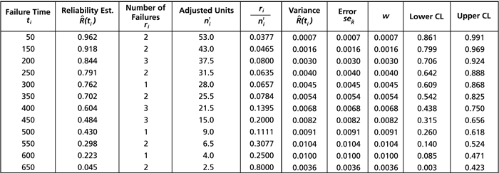
Determine the 1-sided confidence bounds for the reliability estimates in the Actuarial-Simple example, with a 95% confidence level.
Solution
Once again, this type of problem is most readily solved by constructing a table similar to the following:
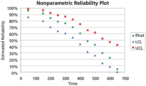
The following plot illustrates these results graphically:
The Weibull++ warranty analysis folio provides four different data entry formats for warranty claims data. It allows the user to automatically perform life data analysis, predict future failures (through the use of conditional probability analysis), and provides a method for detecting outliers. The four data-entry formats for storing sales and returns information are:
- 1) Nevada Chart Format
- 2) Time-to-Failure Format
- 3) Dates of Failure Format
- 4) Usage Format
These formats are explained in the next sections. We will also discuss some specific warranty analysis calculations, including warranty predictions, analysis of non-homogeneous warranty data and using statistical process control (SPC) to monitor warranty returns.
Nevada Chart Format
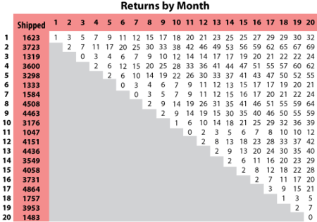
The Nevada format allows the user to convert shipping and warranty return data into the standard reliability data form of failures and suspensions so that it can easily be analyzed with traditional life data analysis methods. For each time period in which a number of products are shipped, there will be a certain number of returns or failures in subsequent time periods, while the rest of the population that was shipped will continue to operate in the following time periods. For example, if 500 units are shipped in May, and 10 of those units are warranty returns in June, that is equivalent to 10 failures at a time of one month. The other 490 units will go on to operate and possibly fail in the months that follow. This information can be arranged in a diagonal chart, as shown in the following figure.
At the end of the analysis period, all of the units that were shipped and have not failed in the time since shipment are considered to be suspensions. This process is repeated for each shipment and the results tabulated for each particular failure and suspension time prior to reliability analysis. This process may sound confusing, but it is actually just a matter of careful bookkeeping. The following example illustrates this process.
Example
Nevada Chart Format Calculations Example
A company keeps track of its shipments and warranty returns on a month-by-month basis. The following table records the shipments in June, July and August, and the warranty returns through September:
| RETURNS | ||||
| SHIP | Jul. 2010 | Aug. 2010 | Sep. 2010 | |
| Jun. 2010 | 100 | 3 | 3 | 5 |
| Jul. 2010 | 140 | - | 2 | 4 |
| Aug. 2010 | 150 | - | - | 4 |
We will examine the data month by month. In June 100 units were sold, and in July 3 of these units were returned. This gives 3 failures at one month for the June shipment, which we will denote as [math]\displaystyle{ {{F}_{JUN,1}}=3\,\! }[/math]. Likewise, 3 failures occurred in August and 5 occurred in September for this shipment, or [math]\displaystyle{ {{F}_{JUN,2}}=3\,\! }[/math] and [math]\displaystyle{ {{F}_{JUN,3}}=5\,\! }[/math]. Consequently, at the end of our three-month analysis period, there were a total of 11 failures for the 100 units shipped in June. This means that 89 units are presumably still operating, and can be considered suspensions at three months, or [math]\displaystyle{ {{S}_{JUN,3}}=89\,\! }[/math]. For the shipment of 140 in July, 2 were returned the following month, or [math]\displaystyle{ {{F}_{JUL,1}}=2\,\! }[/math], and 4 more were returned the month after that, or [math]\displaystyle{ {{F}_{JUL,2}}=4\,\! }[/math]. After two months, there are 134 ( [math]\displaystyle{ 140-2-4=134\,\! }[/math] ) units from the July shipment still operating, or [math]\displaystyle{ {{S}_{JUL,2}}=134\,\! }[/math]. For the final shipment of 150 in August, 4 fail in September, or [math]\displaystyle{ {{F}_{AUG,1}}=4\,\! }[/math], with the remaining 146 units being suspensions at one month, or [math]\displaystyle{ {{S}_{AUG,1}}=146\,\! }[/math].
It is now a simple matter to add up the number of failures for 1, 2, and 3 months, then add the suspensions to get our reliability data set:
These calculations can be performed automatically in Weibull++.
Time-to-Failure Format
This format is similar to the standard folio data entry format (all number of units, failure times and suspension times are entered by the user). The difference is that when the data is used within the context of warranty analysis, the ability to generate forecasts is available to the user.
Example
Times-to-Failure Format Warranty Analysis
Assume that we have the following information for a given product.
| Number in State | State F or S | State End Time (Hr) |
| 2 | F | 100 |
| 3 | F | 125 |
| 5 | F | 175 |
| 1500 | S | 200 |
| Quantity In-Service | Time (Hr) |
| 500 | 200 |
| 400 | 300 |
| 100 | 500 |
Use the time-to-failure warranty analysis folio to analyze the data and generate a forecast for future returns.
Solution
Create a warranty analysis folio and select the times-to-failure format. Enter the data from the tables in the Data and Future Sales sheets, and then analyze the data using the 2P-Weibull distribution and RRX analysis method. The parameters are estimated to be beta = 3.199832 and eta=814.293442.
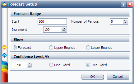
Click the Forecast icon on the control panel. In the Forecast Setup window, set the forecast to start on the 100th hour and set the number of forecast periods to 5. Set the increment (length of each period) to 100, as shown next.
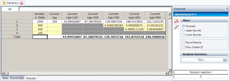
Click OK. A Forecast sheet will be created, with the following predicted future returns.
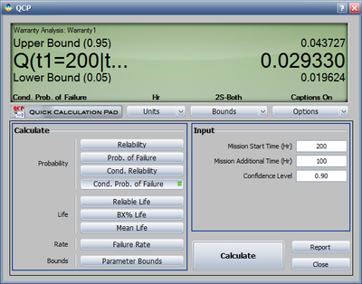
We will use the first row to explain how the forecast for each cell is calculated. For example, there are 1,500 units with a current age of 200 hours. The probability of failure in the next 100 hours can be calculated in the QCP, as follows.
Therefore, the predicted number of failures for the first 100 hours is:
- [math]\displaystyle{ 1500\times 0.02932968=43.99452\,\! }[/math]
This is identical to the result given in the Forecast sheet (shown in the 3rd cell in the first row) of the analysis. The bounds and the values in other cells can be calculated similarly.
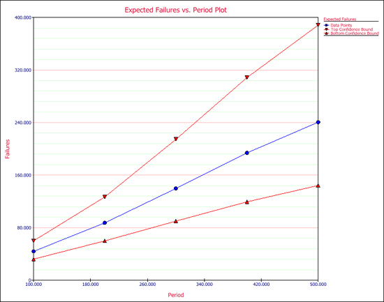
All the plots that are available for the standard folio are also available in the warranty analysis, such as the Probability plot, Reliability plot, etc. One additional plot in warranty analysis is the Expected Failures plot, which shows the expected number of failures over time. The following figure shows the Expected Failures plot of the example, with confidence bounds.
Dates of Failure Format
Another common way for reporting field information is to enter a date and quantity of sales or shipments (Quantity In-Service data) and the date and quantity of returns (Quantity Returned data). In order to identify which lot the unit comes from, a failure is identified by a return date and the date of when it was put in service. The date that the unit went into service is then associated with the lot going into service during that time period. You can use the optional Subset ID column in the data sheet to record any information to identify the lots.
Example
Dates of Failure Warranty Analysis
Assume that a company has the following information for a product.
| Quantity In-Service | Date In-Service |
| 6316 | 1/1/2010 |
| 8447 | 2/1/2010 |
| 5892 | 3/1/2010 |
| 596 | 4/1/2010 |
| 996 | 5/1/2010 |
| 8977 | 6/1/2010 |
| 2578 | 7/1/2010 |
| 8318 | 8/1/2010 |
| 2667 | 9/1/2010 |
| 7452 | 10/1/2010 |
| 1533 | 11/1/2010 |
| 9393 | 12/1/2010 |
| 1966 | 1/1/2011 |
| 8960 | 2/1/2011 |
| 6341 | 3/1/2011 |
| 4005 | 4/1/2011 |
| 3784 | 5/1/2011 |
| 5426 | 6/1/2011 |
| 4958 | 7/1/2011 |
| 6981 | 8/1/2011 |
| Quantity Returned | Date of Return | Date In-Service |
| 2 | 10/29/2010 | 10/1/2010 |
| 1 | 11/13/2010 | 10/1/2010 |
| 2 | 3/15/2011 | 10/1/2010 |
| 5 | 4/10/2011 | 10/1/2010 |
| 1 | 11/13/2010 | 11/1/2010 |
| 2 | 2/19/2011 | 11/1/2010 |
| 1 | 3/11/2011 | 11/1/2010 |
| 2 | 5/18/2011 | 11/1/2010 |
| 1 | 1/9/2011 | 12/1/2010 |
| 2 | 2/13/2011 | 12/1/2010 |
| 1 | 3/2/2011 | 12/1/2010 |
| 1 | 6/7/2011 | 12/1/2010 |
| 1 | 4/28/2011 | 1/1/2011 |
| 2 | 6/15/2011 | 1/1/2011 |
| 3 | 7/15/2011 | 1/1/2011 |
| 1 | 8/10/2011 | 2/1/2011 |
| 1 | 8/12/2011 | 2/1/2011 |
| 1 | 8/14/2011 | 2/1/2011 |
| Quantity In-Service | Date In-Service |
| 5000 | 9/1/2011 |
| 5000 | 10/1/2011 |
| 5000 | 11/1/2011 |
| 5000 | 12/1/2011 |
| 5000 | 1/1/2012 |
Using the given information to estimate the failure distribution of the product and forecast warranty returns.
Solution
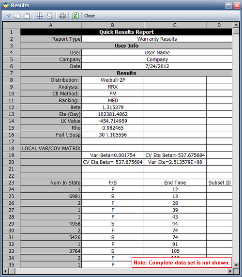
Create a warranty analysis folio using the dates of failure format. Enter the data from the tables in the Sales, Returns and Future Sales sheets. On the control panel, click the Auto-Set button to automatically set the end date to the last day the warranty data were collected (September 14, 2011). Analyze the data using the 2P-Weibull distribution and RRX analysis method. The parameters are estimated to be beta = 1.315379 and eta = 102,381.486165.
The warranty folio automatically converts the warranty data into a format that can be used in a Weibull++ standard folio. To see this result, click anywhere within the Analysis Summary area of the control panel to open a report, as shown next (showing only the first 35 rows of data). In this example, rows 23 to 60 show the time-to-failure data that resulted from the conversion.
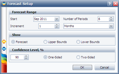
To generate a forecast, click the Forecast icon on the control panel. In the Forecast Setup window, set the forecast to start on September 2011 and set the number of forecast periods to 6. Set the increment (length of each period) to 1 Month, as shown next.
Click OK. A Forecast sheet will be created, with the predicted future returns. Note that the first forecast will start on September 15, 2011 because the end of observation period was set to September 14, 2011.
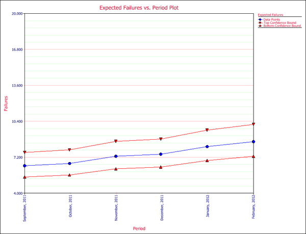
Click the Plot icon and choose the Expected Failures plot. The plot displays the predicted number of returns for each month, as shown next.
Usage Format
Often, the driving factor for reliability is usage rather than time. For example, in the automotive industry, the failure behavior in the majority of the products is mileage-dependent rather than time-dependent. The usage format allows the user to convert shipping and warranty return data into the standard reliability data for of failures and suspensions when the return information is based on usage rather than return dates or periods. Similar to the dates of failure format, a failure is identified by the return number and the date of when it was put in service in order to identify which lot the unit comes from. The date that the returned unit went into service associates the returned unit with the lot it belonged to when it started operation. However, the return data is in terms of usage and not date of return. Therefore the usage of the units needs to be specified as a constant usage per unit time or as a distribution. This allows for determining the expected usage of the surviving units.
Suppose that you have been collecting sales (units in service) and returns data. For the returns data, you can determine the number of failures and their usage by reading the odometer value, for example. Determining the number of surviving units (suspensions) and their ages is a straightforward step. By taking the difference between the analysis date and the date when a unit was put in service, you can determine the age of the surviving units.
What is unknown, however, is the exact usage accumulated by each surviving unit. The key part of the usage-based warranty analysis is the determination of the usage of the surviving units based on their age. Therefore, the analyst needs to have an idea about the usage of the product. This can be obtained, for example, from customer surveys or by designing the products to collect usage data. For example, in automotive applications, engineers often use 12,000 miles/year as the average usage. Based on this average, the usage of an item that has been in the field for 6 months and has not yet failed would be 6,000 miles. So to obtain the usage of a suspension based on an average usage, one could take the time of each suspension and multiply it by this average usage. In this situation, the analysis becomes straightforward. With the usage values and the quantities of the returned units, a failure distribution can be constructed and subsequent warranty analysis becomes possible.
Alternatively, and more realistically, instead of using an average usage, an actual distribution that reflects the variation in usage and customer behavior can be used. This distribution describes the usage of a unit over a certain time period (e.g., 1 year, 1 month, etc). This probabilistic model can be used to estimate the usage for all surviving components in service and the percentage of users running the product at different usage rates. In the automotive example, for instance, such a distribution can be used to calculate the percentage of customers that drive 0-200 miles/month, 200-400 miles/month, etc. We can take these percentages and multiply them by the number of suspensions to find the number of items that have been accumulating usage values in these ranges.
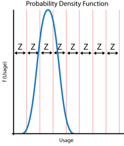
To proceed with applying a usage distribution, the usage distribution is divided into increments based on a specified interval width denoted as [math]\displaystyle{ Z\,\! }[/math]. The usage distribution, [math]\displaystyle{ Q\,\! }[/math], is divided into intervals of [math]\displaystyle{ 0+Z\,\! }[/math], [math]\displaystyle{ Z+Z\,\! }[/math], [math]\displaystyle{ 2Z+Z\,\! }[/math], etc., or [math]\displaystyle{ {{x}_{i}}={{x}_{i-1}}+Z\,\! }[/math], as shown in the next figure.
The interval width should be selected such that it creates segments that are large enough to contain adequate numbers of suspensions within the intervals. The percentage of suspensions that belong to each usage interval is calculated as follows:
- [math]\displaystyle{ \begin{align} F({{x}_{i}})=Q({{x}_{i}})-Q({{x}_{i}}-1) \end{align}\,\! }[/math]
where:
- [math]\displaystyle{ Q()\,\! }[/math] is the usage distribution Cumulative Density Function, cdf.
- [math]\displaystyle{ x\,\! }[/math] represents the intervals used in apportioning the suspended population.
A suspension group is a collection of suspensions that have the same age. The percentage of suspensions can be translated to numbers of suspensions within each interval, [math]\displaystyle{ {{x}_{i}}\,\! }[/math]. This is done by taking each group of suspensions and multiplying it by each [math]\displaystyle{ F({{x}_{i}})\,\! }[/math], or:
- [math]\displaystyle{ \begin{align} & {{N}_{1,j}}= & F({{x}_{1}})\times N{{S}_{j}} \\ & {{N}_{2,j}}= & F({{x}_{2}})\times N{{S}_{j}} \\ & & ... \\ & {{N}_{n,j}}= & F({{x}_{n}})\times N{{S}_{j}} \end{align}\,\! }[/math]
where:
- [math]\displaystyle{ {{N}_{n,j}}\,\! }[/math] is the number of suspensions that belong to each interval.
- [math]\displaystyle{ N{{S}_{j}}\,\! }[/math] is the jth group of suspensions from the data set.
This is repeated for all the groups of suspensions.
The age of the suspensions is calculated by subtracting the Date In-Service ( [math]\displaystyle{ DIS\,\! }[/math] ), which is the date at which the unit started operation, from the end of observation period date or End Date ( [math]\displaystyle{ ED\,\! }[/math] ). This is the Time In-Service ( [math]\displaystyle{ TIS\,\! }[/math] ) value that describes the age of the surviving unit.
- [math]\displaystyle{ \begin{align} TIS=ED-DIS \end{align}\,\! }[/math]
Note: [math]\displaystyle{ TIS\,\! }[/math] is in the same time units as the period in which the usage distribution is defined.
For each [math]\displaystyle{ {{N}_{k,j}}\,\! }[/math], the usage is calculated as:
- [math]\displaystyle{ Uk,j=xi\times TISj\,\! }[/math]
After this step, the usage of each suspension group is estimated. This data can be combined with the failures data set, and a failure distribution can be fitted to the combined data.
Example
Warranty Analysis Usage Format Example
Suppose that an automotive manufacturer collects the warranty returns and sales data given in the following tables. Convert this information to life data and analyze it using the lognormal distribution.
| Quantity In-Service | Date In-Service |
| 9 | Dec-09 |
| 13 | Jan-10 |
| 15 | Feb-10 |
| 20 | Mar-10 |
| 15 | Apr-10 |
| 25 | May-10 |
| 19 | Jun-10 |
| 16 | Jul-10 |
| 20 | Aug-10 |
| 19 | Sep-10 |
| 25 | Oct-10 |
| 30 | Nov-10 |
| Quantity Returned | Usage at Return Date | Date In-Service |
| 1 | 9072 | Dec-09 |
| 1 | 9743 | Jan-10 |
| 1 | 6857 | Feb-10 |
| 1 | 7651 | Mar-10 |
| 1 | 5083 | May-10 |
| 1 | 5990 | May-10 |
| 1 | 7432 | May-10 |
| 1 | 8739 | May-10 |
| 1 | 3158 | Jun-10 |
| 1 | 1136 | Jul-10 |
| 1 | 4646 | Aug-10 |
| 1 | 3965 | Sep-10 |
| 1 | 3117 | Oct-10 |
| 1 | 3250 | Nov-10 |
Solution
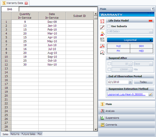
Create a warranty analysis folio and select the usage format. Enter the data from the tables in the Sales, Returns and Future Sales sheets. The warranty data were collected until 12/1/2010; therefore, on the control panel, set the End of Observation Period to that date. Set the failure distribution to Lognormal, as shown next.
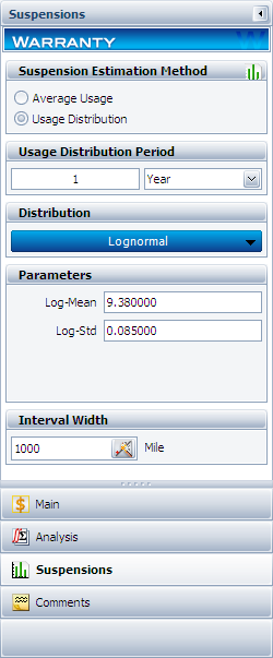
In this example, the manufacturer has been documenting the mileage accumulation per year for this type of product across the customer base in comparable regions for many years. The yearly usage has been determined to follow a lognormal distribution with [math]\displaystyle{ {{\mu }_{T\prime }}=9.38\,\! }[/math], [math]\displaystyle{ {{\sigma }_{T\prime }}=0.085\,\! }[/math]. The Interval Width is defined to be 1,000 miles. Enter the information about the usage distribution on the Suspensions page of the control panel, as shown next.
Click Calculate to analyze the data set. The parameters are estimated to be:
- [math]\displaystyle{ \begin{align} & {{\mu }_{T\prime }}= & 10.528098 \\ & {{\sigma }_{T\prime }}= & 1.135150 \end{align}\,\! }[/math]
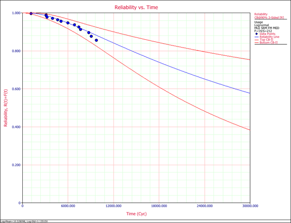
The reliability plot (with mileage being the random variable driving reliability), along with the 90% confidence bounds on reliability, is shown next.
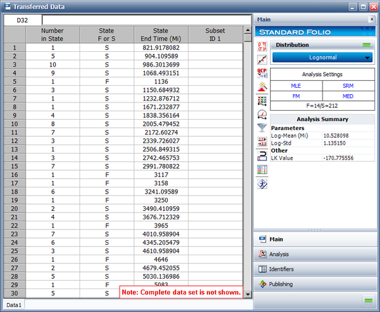
In this example, the life data set contains 14 failures and 212 suspensions spread according to the defined usage distribution. You can display this data in a standard folio by choosing Warranty > Transfer Life Data > Transfer Life Data to New Folio. The failures and suspensions data set, as presented in the standard folio, is shown next (showing only the first 30 rows of data).
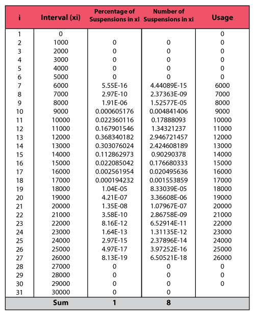
To illustrate the calculations behind the results of this example, consider the 9 units that went in service on December 2009. 1 unit failed from that group; therefore, 8 suspensions have survived from December 2009 until the beginning of December 2010, a total of 12 months. The calculations are summarized as follows.
The two columns on the right constitute the calculated suspension data (number of suspensions and their usage) for the group. The calculation is then repeated for each of the remaining groups in the data set. These data are then combined with the data about the failures to form the life data set that is used to estimate the failure distribution model.
Warranty Prediction
Once a life data analysis has been performed on warranty data, this information can be used to predict how many warranty returns there will be in subsequent time periods. This methodology uses the concept of conditional reliability (see Basic Statistical Background) to calculate the probability of failure for the remaining units for each shipment time period. This conditional probability of failure is then multiplied by the number of units at risk from that particular shipment period that are still in the field (i.e., the suspensions) in order to predict the number of failures or warranty returns expected for this time period. The next example illustrates this.
Example
Using the data in the following table, predict the number of warranty returns for October for each of the three shipment periods. Use the following Weibull parameters, beta = 2.4928 and eta = 6.6951.
| RETURNS | ||||
| SHIP | Jul. 2010 | Aug. 2010 | Sep. 2010 | |
| Jun. 2010 | 100 | 3 | 3 | 5 |
| Jul. 2010 | 140 | - | 2 | 4 |
| Aug. 2010 | 150 | - | - | 4 |
Solution
Use the Weibull parameter estimates to determine the conditional probability of failure for each shipment time period, and then multiply that probability with the number of units that are at risk for that period as follows. The equation for the conditional probability of failure is given by:
- [math]\displaystyle{ Q(t|T)=1-R(t|T)=1-\frac{R(T+t)}{R(T)}\,\! }[/math]
For the June shipment, there are 89 units that have successfully operated until the end of September ( [math]\displaystyle{ T=3 months)\,\! }[/math]. The probability of one of these units failing in the next month ( [math]\displaystyle{ t=1 month)\,\! }[/math] is then given by:
- [math]\displaystyle{ Q(1|3)=1-\frac{R(4)}{R(3)}=1-\frac{{{e}^{-{{\left( \tfrac{4}{6.70} \right)}^{2.49}}}}}{{{e}^{-{{\left( \tfrac{3}{6.70} \right)}^{2.49}}}}}=1-\frac{0.7582}{0.8735}=0.132\,\! }[/math]
Once the probability of failure for an additional month of operation is determined, the expected number of failed units during the next month, from the June shipment, is the product of this probability and the number of units at risk ( [math]\displaystyle{ {{S}_{JUN,3}}=89)\,\! }[/math] or:
- [math]\displaystyle{ {{\widehat{F}}_{JUN,4}}=89\cdot 0.132=11.748\text{, or 12 units}\,\! }[/math]
This is then repeated for the July shipment, where there were 134 units operating at the end of September, with an exposure time of two months. The probability of failure in the next month is:
- [math]\displaystyle{ Q(1|2)=1-\frac{R(3)}{R(2)}=1-\frac{0.8735}{0.9519}=0.0824\,\! }[/math]
This value is multiplied by [math]\displaystyle{ {{S}_{JUL,2}}=134\,\! }[/math] to determine the number of failures, or:
- [math]\displaystyle{ {{\widehat{F}}_{JUL,3}}=134\cdot 0.0824=11.035\text{, or 11 units}\,\! }[/math]
For the August shipment, there were 146 units operating at the end of September, with an exposure time of one month. The probability of failure in the next month is:
- [math]\displaystyle{ Q(1|1)=1-\frac{R(2)}{R(1)}=1-\frac{0.9519}{0.9913}=0.0397\,\! }[/math]
This value is multiplied by [math]\displaystyle{ {{S}_{AUG,1}}=146\,\! }[/math] to determine the number of failures, or:
- [math]\displaystyle{ {{\widehat{F}}_{AUG,2}}=146\cdot 0.0397=5.796\text{, or 6 units}\,\! }[/math]
Thus, the total expected returns from all shipments for the next month is the sum of the above, or 29 units. This method can be easily repeated for different future sales periods, and utilizing projected shipments. If the user lists the number of units that are expected be sold or shipped during future periods, then these units are added to the number of units at risk whenever they are introduced into the field. The Generate Forecast functionality in the Weibull++ warranty analysis folio can automate this process for you.
Non-Homogeneous Warranty Data
In the previous sections and examples, it is important to note that the underlying assumption was that the population was homogeneous. In other words, all sold and returned units were exactly the same (i.e., the same population with no design changes and/or modifications). In many situations, as the product matures, design changes are made to enhance and/or improve the reliability of the product. Obviously, an improved product will exhibit different failure characteristics than its predecessor. To analyze such cases, where the population is non-homogeneous, one needs to extract each homogenous group, fit a life model to each group and then project the expected returns for each group based on the number of units at risk for each specific group.
Using Subset IDs in Weibull++
Weibull++ includes an optional Subset ID column that allows to differentiate between product versions or different designs (lots). Based on the entries, the software will separately analyze (i.e., obtain parameters and failure projections for) each subset of data. Note that it is important to realize that the same limitations with regards to the number of failures that are needed are also applicable here. In other words, distributions can be automatically fitted to lots that have return (failure) data, whereas if no returns have been experienced yet (either because the units are going to be introduced in the future or because no failures happened yet), the user will be asked to specify the parameters, since they can not be computed. Consequently, subsequent estimation/predictions related to these lots would be based on the user specified parameters. The following example illustrates the use of Subset IDs.
Example
Warranty Analysis Non-Homogeneous Data Example
A company keeps track of its production and returns. The company uses the dates of failure format to record the data. For the product in question, three versions (A, B and C) have been produced and put in service. The in-service data is as follows (using the Month/Day/Year date format):
Furthermore, the following sales are forecast:
The return data are as follows. Note that in order to identify which lot each unit comes from, and to be able to compute its time-in-service, each return (failure) includes a return date, the date of when it was put in service and the model ID.
Assuming that the given information is current as of 5/1/2006, analyze the data using the lognormal distribution and MLE analysis method for all models (Model A, Model B, Model C), and provide a return forecast for the next ten months.
Solution
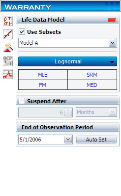
Create a warranty analysis folio and select the dates of failure format. Enter the data from the tables in the Sales, Returns and Future Sales sheets. On the control panel, select the Use Subsets check box, as shown next. This allows the software to separately analyze each subset of data. Use the drop-down list to switch between subset IDs and alter the analysis settings (use the lognormal distribution and MLE analysis method for all models).
In the End of Observation Period field, enter 5/1/2006, and then calculate the parameters. The results are:
Note that in this example, the same distribution and analysis method were assumed for each of the product models. If desired, different distribution types, analysis methods, confidence bounds methods, etc., can be assumed for each IDs.
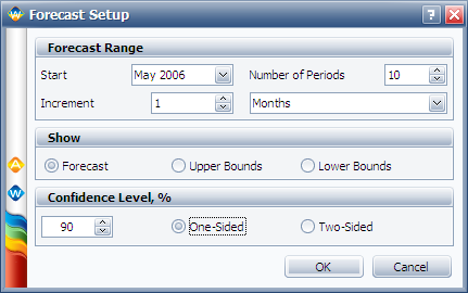
To obtain the expected failures for the next 10 months, click the Generate Forecast icon. In the Forecast Setup window, set the forecast to start on May 2, 2006 and set the number of forecast periods to 10. Set the increment (length of each period) to 1 Month, as shown next.
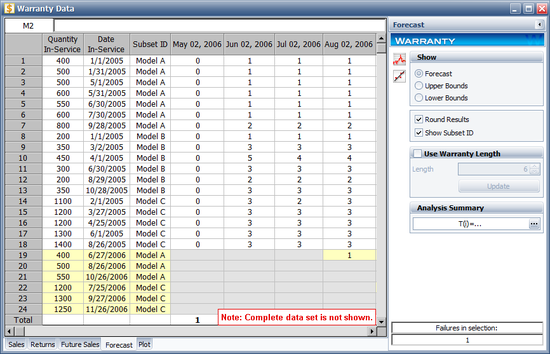
Click OK. A Forecast sheet will be created, with the predicted future returns. The following figure shows part of the Forecast sheet.
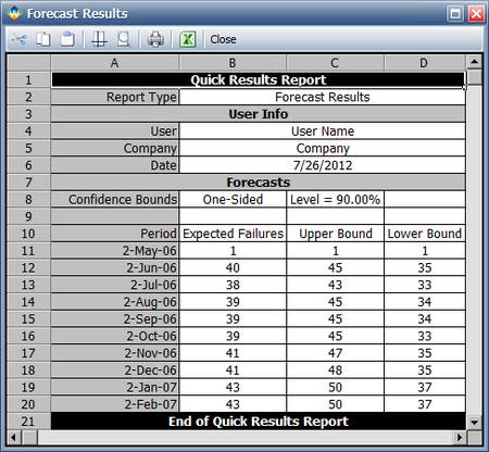
To view a summary of the analysis, click the Show Analysis Summary (...) button. The following figure shows the summary of the forecasted returns.
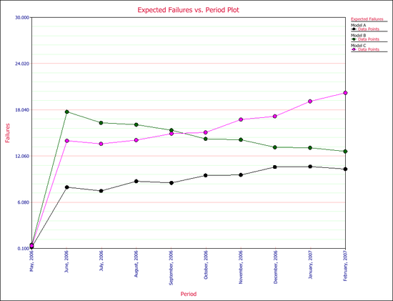
Click the Plot icon and choose the Expected Failures plot. The plot displays the predicted number of returns for each month, as shown next.
Monitoring Warranty Returns Using Statistical Process Control (SPC)
By monitoring and analyzing warranty return data, one can detect specific return periods and/or batches of sales or shipments that may deviate (differ) from the assumed model. This provides the analyst (and the organization) the advantage of early notification of possible deviations in manufacturing, use conditions and/or any other factor that may adversely affect the reliability of the fielded product. Obviously, the motivation for performing such analysis is to allow for faster intervention to avoid increased costs due to increased warranty returns or more serious repercussions. Additionally, this analysis can also be used to uncover different sub-populations that may exist within the population.
Basic Analysis Method
For each sales period [math]\displaystyle{ i\,\! }[/math] and return period [math]\displaystyle{ j\,\! }[/math], the prediction error can be calculated as follows:
- [math]\displaystyle{ {{e}_{i,j}}={{\hat{F}}_{i,j}}-{{F}_{i,j}}\,\! }[/math]
where [math]\displaystyle{ {{\hat{F}}_{i,j}}\,\! }[/math] is the estimated number of failures based on the estimated distribution parameters for the sales period [math]\displaystyle{ i\,\! }[/math] and the return period [math]\displaystyle{ j\,\! }[/math], which is calculated using the equation for the conditional probability, and [math]\displaystyle{ {{F}_{i,j}}\,\! }[/math] is the actual number of failure for the sales period [math]\displaystyle{ i\,\! }[/math] and the return period [math]\displaystyle{ j\,\! }[/math].
Since we are assuming that the model is accurate, [math]\displaystyle{ {{e}_{i,j}}\,\! }[/math] should follow a normal distribution with mean value of zero and a standard deviation [math]\displaystyle{ s\,\! }[/math], where:
- [math]\displaystyle{ {{\bar{e}}_{i,j}}=\frac{\underset{i}{\mathop{\sum }}\,\underset{j}{\mathop{\sum }}\,{{e}_{i,j}}}{n}=0\,\! }[/math]
and [math]\displaystyle{ n\,\! }[/math] is the total number of return data (total number of residuals).
The estimated standard deviation of the prediction errors can then be calculated by:
- [math]\displaystyle{ s=\sqrt{\frac{1}{n-1}\underset{i}{\mathop \sum }\,\underset{j}{\mathop \sum }\,e_{i,j}^{2}}\,\! }[/math]
and [math]\displaystyle{ {{e}_{i,j}}\,\! }[/math] can be normalized as follows:
- [math]\displaystyle{ {{z}_{i,j}}=\frac{{{e}_{i,j}}}{s}\,\! }[/math]
where [math]\displaystyle{ {{z}_{i,j}}\,\! }[/math] is the standardized error. [math]\displaystyle{ {{z}_{i,j}}\,\! }[/math] follows a normal distribution with [math]\displaystyle{ \mu =0\,\! }[/math] and [math]\displaystyle{ \sigma =1\,\! }[/math].
It is known that the square of a random variable with standard normal distribution follows the [math]\displaystyle{ {{\chi }^{2}}\,\! }[/math] (Chi Square) distribution with 1 degree of freedom and that the sum of the squares of [math]\displaystyle{ m\,\! }[/math] random variables with standard normal distribution follows the [math]\displaystyle{ {{\chi }^{2}}\,\! }[/math] distribution with [math]\displaystyle{ m\,\! }[/math] degrees of freedom. This then can be used to help detect the abnormal returns for a given sales period, return period or just a specific cell (combination of a return and a sales period).
- For a cell, abnormality is detected if [math]\displaystyle{ z_{i,j}^{2}=\chi _{1}^{2}\ge \chi _{1,\alpha }^{2}.\,\! }[/math]
- For an entire sales period [math]\displaystyle{ i\,\! }[/math], abnormality is detected if [math]\displaystyle{ \underset{j}{\mathop{\sum }}\,z_{i,j}^{2}=\chi _{J}^{2}\ge \chi _{\alpha ,J}^{2},\,\! }[/math] where [math]\displaystyle{ J\,\! }[/math] is the total number of return period for a sales period [math]\displaystyle{ i\,\! }[/math].
- For an entire return period [math]\displaystyle{ j\,\! }[/math], abnormality is detected if [math]\displaystyle{ \underset{i}{\mathop{\sum }}\,z_{i,j}^{2}=\chi _{I}^{2}\ge \chi _{\alpha ,I}^{2},\,\! }[/math] where [math]\displaystyle{ I\,\! }[/math] is the total number of sales period for a return period [math]\displaystyle{ j\,\! }[/math].
Here [math]\displaystyle{ \alpha \,\! }[/math] is the criticality value of the [math]\displaystyle{ {{\chi }^{2}}\,\! }[/math] distribution, which can be set at critical value or caution value. It describes the level of sensitivity to outliers (returns that deviate significantly from the predictions based on the fitted model). Increasing the value of [math]\displaystyle{ \alpha \,\! }[/math] increases the power of detection, but this could lead to more false alarms.
Example
Example Using SPC for Warranty Analysis Data
Using the data from the following table, the expected returns for each sales period can be obtained using conditional reliability concepts, as given in the conditional probability equation.
| RETURNS | ||||
| SHIP | Jul. 2010 | Aug. 2010 | Sep. 2010 | |
| Jun. 2010 | 100 | 3 | 3 | 5 |
| Jul. 2010 | 140 | - | 2 | 4 |
| Aug. 2010 | 150 | - | - | 4 |
For example, for the month of September, the expected return number from the June shipment is given by:
- [math]\displaystyle{ {{\hat{F}}_{Jun,3}}=(100-6)\cdot \left( 1-\frac{R(3)}{R(2)} \right)=94\cdot 0.08239=7.7447\,\! }[/math]
The actual number of returns during this period is five; thus, the prediction error for this period is:
- [math]\displaystyle{ {{e}_{Jun,3}}={{\hat{F}}_{Jun,3}}-{{F}_{Jun,3}}=7.7447-5=2.7447.\,\! }[/math]
This can then be repeated for each cell, yielding the following table for [math]\displaystyle{ {{e}_{i,j}}\,\! }[/math] :
Now, for this example, [math]\displaystyle{ n=6\,\! }[/math], [math]\displaystyle{ {{\bar{e}}_{i,j}}=-0.0904\,\! }[/math] and [math]\displaystyle{ s=2.1366.\,\! }[/math]
Thus the [math]\displaystyle{ z_{i,j}\,\! }[/math] values are:
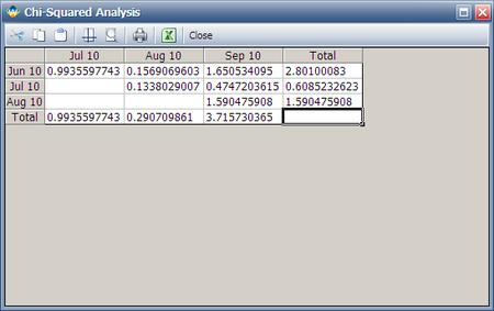
The [math]\displaystyle{ z_{i,j}^{2}\,\! }[/math] values, for each cell, are given in the following table.
If the critical value is set at [math]\displaystyle{ \alpha = 0.01\,\! }[/math] and the caution value is set at [math]\displaystyle{ \alpha = 0.1\,\! }[/math], then the critical and caution [math]\displaystyle{ {{\chi }^{2}}\,\! }[/math] values will be:
If we consider the sales periods as the basis for outlier detection, then after comparing the above table to the sum of [math]\displaystyle{ z_{i,j}^{2}\,\! }[/math] [math]\displaystyle{ (\chi _{1}^{2})\,\! }[/math] values for each sales period, we find that all the sales values do not exceed the critical and caution limits. For example, the total [math]\displaystyle{ {{\chi }^{2}}\,\! }[/math] value of the sale month of July is 0.6085. Its degrees of freedom is 2, so the corresponding caution and critical values are 4.6052 and 9.2103 respectively. Both values are larger than 0.6085, so the return numbers of the July sales period do not deviate (based on the chosen significance) from the model's predictions.
If we consider returns periods as the basis for outliers detection, then after comparing the above table to the sum of [math]\displaystyle{ z_{i,j}^{2}\,\! }[/math] [math]\displaystyle{ (\chi _{1}^{2})\,\! }[/math] values for each return period, we find that all the return values do not exceed the critical and caution limits. For example, the total [math]\displaystyle{ {{\chi }^{2}}\,\! }[/math] value of the sale month of August is 3.7157. Its degree of freedom is 3, so the corresponding caution and critical values are 6.2514 and 11.3449 respectively. Both values are larger than 3.7157, so the return numbers for the June return period do not deviate from the model's predictions.
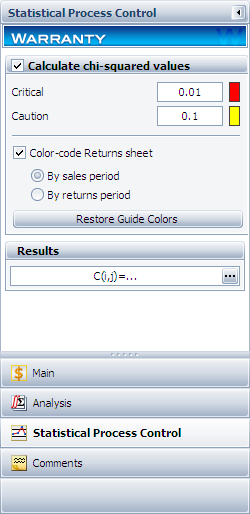
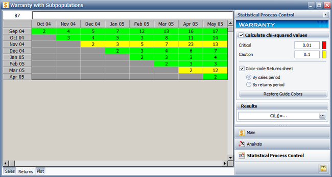
This analysis can be automatically performed in Weibull++ by entering the alpha values in the Statistical Process Control page of the control panel and selecting which period to color code, as shown next.
To view the table of chi-squared values ( [math]\displaystyle{ z_{i,j}^{2}\,\! }[/math] or [math]\displaystyle{ \chi _{1}^{2}\,\! }[/math] values), click the Show Results (...) button.
Weibull++ automatically color codes SPC results for easy visualization in the returns data sheet. By default, the green color means that the return number is normal; the yellow color indicates that the return number is larger than the caution threshold but smaller than the critical value; the red color means that the return is abnormal, meaning that the return number is either too big or too small compared to the predicted value.
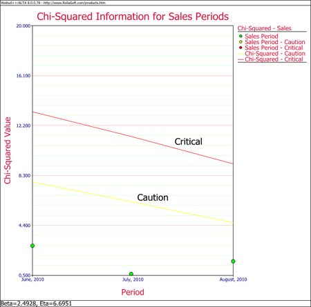
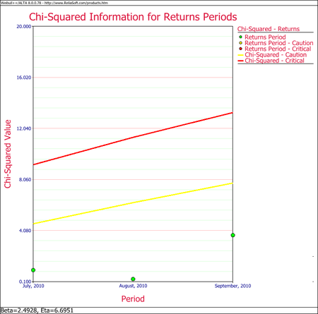
In this example, all the cells are coded in green for both analyses (i.e., by sales periods or by return periods), indicating that all returns fall within the caution and critical limits (i.e., nothing abnormal). Another way to visualize this is by using a Chi-Squared plot for the sales period and return period, as shown next.
Using Subset IDs with SPC for Warranty Data
The warranty monitoring methodology explained in this section can also be used to detect different subpopulations in a data set. The different subpopulations can reflect different use conditions, different material, etc. In this methodology, one can use different subset IDs to differentiate between subpopulations, and obtain models that are distinct to each subpopulation. The following example illustrates this concept.
Example
Using Subset IDs with Statistical Process Control
A manufacturer wants to monitor and analyze the warranty returns for a particular product. They collected the following sales and return data.
Solution
Analyze the data using the two-parameter Weibull distribution and the MLE analysis method. The parameters are estimated to be:
- [math]\displaystyle{ \begin{align} & & \beta = & 2.318144 \\ & & \eta = & 25.071878 \end{align}\,\! }[/math]
To analyze the warranty returns, select the check box in the Statistical Process Control page of the control panel and set the alpha values to 0.01 for the Critical Value and 0.1 for the Caution Value. Select to color code the results By sales period. The following figure shows the analysis settings and results of the analysis.
As you can see, the November 04 and March 05 sales periods are colored in yellow indicating that they are outlier sales periods, while the rest are green. One suspected reason for the variation may be the material used in production during these periods. Further analysis confirmed that for these periods, the material was acquired from a different supplier. This implies that the units are not homogenous, and that there are different sub-populations present in the field population.
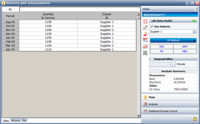
Categorized each shipment (using the Subset ID column) based on their material supplier, as shown next. On the control panel, select the Use Subsets check box. Perform the analysis again using the two-parameter Weibull distribution and the MLE analysis method for both sub-populations.
The new models that describe the data are:
This analysis uncovered different sub-populations in the data set. Note that if the analysis were performed on the failure and suspension times in a regular standard folio using the mixed Weibull distribution, one would not be able to detect which units fall into which sub-population.
The following table gives the failure times for the air conditioning unit of an aircraft. The observation ended by the time the last failure occurred, as discussed in Cox [3].
1. Estimate the GRP model parameters using the Type I virtual age option.
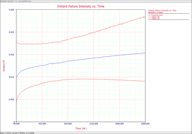
2. Plot the failure number and instantaneous failure intensity vs. time with 90% two-sided confidence bounds.
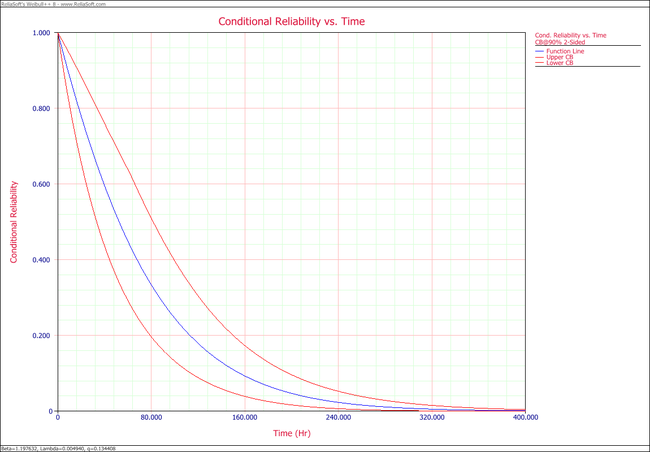
3. Plot the conditional reliability vs. time with 90% two-sided confidence bounds. The mission start time is 40 and mission time is varying.
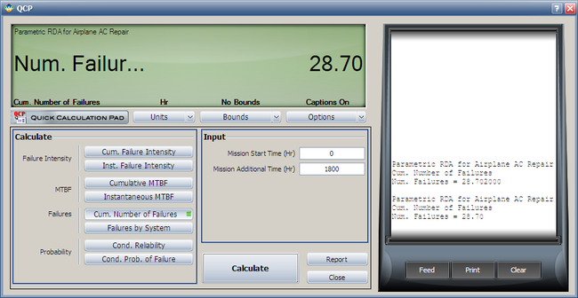
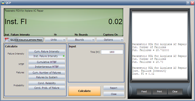
4. Using the QCP, calculate the expected failure number and expected instantaneous failure intensity by time 1800.
Solution
Enter the data into a parametric RDA folio in Weibull++. On the control panel, select the 3 parameters option and the Type I setting. Keep the default simulation settings. Click Calculate.
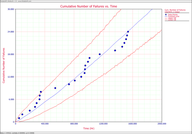
- 1. The estimated parameters are [math]\displaystyle{ \hat{\beta }=1.1976\,\! }[/math], [math]\displaystyle{ \hat{\lambda }=4.94E-03\,\! }[/math], [math]\displaystyle{ \hat{q}=0.1344\,\! }[/math].
- 2. The following plots show the cumulative number of failures and instantaneous failure intensity, respectively.
- 3. The following plot shows the conditional reliability.
- 4. Using the QCP, the failure number and instantaneous failure intensity are:
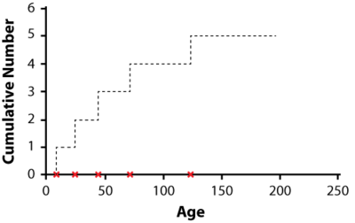
Recurrent Event Data Analysis (RDA) is used in various applied fields such as reliability, medicine, social sciences, economics, business and criminology. Whereas in life data analysis (LDA) it was assumed that events (failures) were independent and identically distributed (iid), there are many cases where events are dependent and not identically distributed (such as repairable system data) or where the analyst is interested in modeling the number of occurrences of events over time rather than the length of time prior to the first event, as in LDA.
Weibull++ provides both parametric and non-parametric approaches to analyze such data.
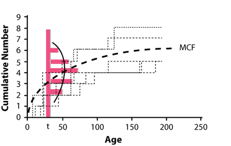
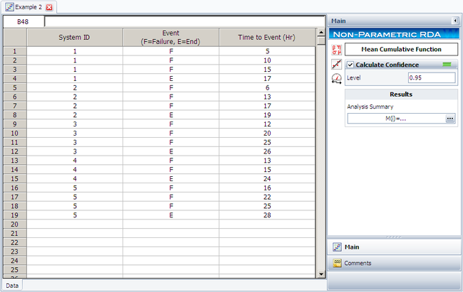
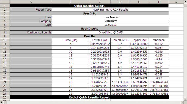
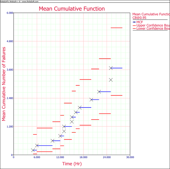
- The non-parametric approach is based on the well-known Mean Cumulative Function (MCF). The Weibull++ module for this type of analysis builds upon the work of Dr. Wayne Nelson, who has written extensively on the calculation and applications of MCF [31].
- The parametric approach is based on the General Renewal Process (GRP) model, which is particularly useful in understanding the effects of the repairs on the age of a system. Traditionally, the commonly used models for analyzing repairable systems data are the perfect renewal processes (PRP), which corresponds to perfect repairs, and the nonhomogeneous Poisson processes (NHPP), which corresponds to minimal repairs. However, most repair activities may realistically not result in such extreme situations but in a complicated intermediate one (general repair or imperfect repair/maintenance), which are well treated with the GRP model.
Non-Parametric Recurrent Event Data Analysis
Parametric Recurrent Event Data Analysis
Weibull++'s parametric RDA folio is a tool for modeling recurrent event data. It can capture the trend, estimate the rate and predict the total number of recurrences. The failure and repair data of a repairable system can be treated as one type of recurrence data. Past and current repairs may affect the future failure process. For most recurrent events, time (distance, cycles, etc.) is a key factor. With time, the recurrence rate may remain constant, increase or decrease. For other recurrent events, not only the time, but also the number of events can affect the recurrence process (e.g., the debugging process in software development).
The parametric analysis approach utilizes the General Renewal Process (GRP) model, as discussed in Mettas and Zhao [28]. In this model, the repair time is assumed to be negligible so that the processes can be viewed as point processes. This model provides a way to describe the rate of occurrence of events over time, such as in the case of data obtained from a repairable system. This model is particularly useful in modeling the failure behavior of a specific system and understanding the effects of the repairs on the age of that system. For example, consider a system that is repaired after a failure, where the repair does not bring the system to an as-good-as-new or an as-bad-as-old condition. In other words, the system is partially rejuvenated after the repair. Traditionally, in as-bad-as-old repairs, also known as minimal repairs, the failure data from such a system would have been modeled using a homogeneous or non-homogeneous Poisson process (NHPP). On rare occasions, a Weibull distribution has been used as well in cases where the system is almost as-good-as-new after the repair, also known as a perfect renewal process (PRP). However, for the intermediate states after the repair, there has not been a commercially available model, even though many models have been proposed in literature. In Weibull++, the GRP model provides the capability to model systems with partial renewal (general repair or imperfect repair/maintenance) and allows for a variety of predictions such as reliability, expected failures, etc.
The GRP Model
In this model, the concept of virtual age is introduced. Let [math]\displaystyle{ {{t}_{1}},{{t}_{2}},\cdots ,{{t}_{n}}\,\! }[/math] represent the successive failure times and let [math]\displaystyle{ {{x}_{1}},{{x}_{2}},\cdots ,{{x}_{n}}\,\! }[/math] represent the time between failures ( [math]\displaystyle{ {{t}_{i}}=\sum_{j=1}^{i}{{x}_{j}})\,\! }[/math]. Assume that after each event, actions are taken to improve the system performance. Let [math]\displaystyle{ q\,\! }[/math] be the action effectiveness factor. There are two GRP models:
Type I:
- [math]\displaystyle{ \begin{align} v_{i}=v_{i-1}+qx_{i}=qt_{i} \end{align}\,\! }[/math]
Type II:
- [math]\displaystyle{ {{v}_{i}}=q({{v}_{i-1}}+{{x}_{i}})={{q}^{i}}{{x}_{1}}+{{q}^{i-1}}{{x}_{2}}+\cdots +{{q}{x}_{i}}\,\! }[/math]
where [math]\displaystyle{ {{v}_{i}}\,\! }[/math] is the virtual age of the system right after [math]\displaystyle{ i\,\! }[/math]th repair. The Type I model assumes that the [math]\displaystyle{ i\,\! }[/math]th repair cannot remove the damage incurred before the [math]\displaystyle{ (i-1)\,\! }[/math] th repair. It can only reduce the additional age [math]\displaystyle{ {{x}_{i}}\,\! }[/math] to [math]\displaystyle{ {{qx}_{i}}\,\! }[/math]. The Type II model assumes that at the [math]\displaystyle{ i\,\! }[/math]th repair, the virtual age has been accumulated to [math]\displaystyle{ v_{i-1} + {{x}_{i}}\,\! }[/math]. The [math]\displaystyle{ i\,\! }[/math]th repair will remove the cumulative damage from both current and previous failures by reducing the virtual age to [math]\displaystyle{ q(v_{i-1} + x_{i})\,\! }[/math].
The power law function is used to model the rate of recurrence, which is:
- [math]\displaystyle{ \begin{align} \lambda(t)=\lambda \beta t^{\beta -1} \end{align}\,\! }[/math]
The conditional pdf is:
- [math]\displaystyle{ f({{t}_{i}}|{{t}_{i-1}})=\lambda \beta {{({{x}_{i}}+{{v}_{i-1}})}^{\beta -1}}{{e}^{-\lambda \left[ {{\left( {{x}_{i}}+{{v}_{i-1}} \right)}^{\beta }}-v_{i-1}^{\beta } \right]}}\,\! }[/math]
MLE method is used to estimate the model parameters. The log likelihood function is discussed in Mettas and Zhao [28]:
- [math]\displaystyle{ \begin{align} & \ln (L)= n(\ln \lambda +\ln \beta )-\lambda \left[ {{\left( T-{{t}_{n}}+{{v}_{n}} \right)}^{\beta }}-v_{n}^{\beta } \right] \\ & -\lambda \underset{i=1}{\overset{n}{\mathop \sum }}\,\left[ {{\left( {{x}_{i}}+{{v}_{i-1}} \right)}^{\beta }}-v_{i-1}^{\beta } \right]+(\beta -1)\underset{i=1}{\overset{n}{\mathop \sum }}\,\ln ({{x}_{i}}+{{v}_{i-1}}) \end{align}\,\! }[/math]
where [math]\displaystyle{ n\,\! }[/math] is the total number of events during the entire observation period. [math]\displaystyle{ T\,\! }[/math] is the stop time of the observation. [math]\displaystyle{ T = t_{n}\,\! }[/math] if the observation stops right after the last event.
Confidence Bounds
In general, in order to obtain the virtual age, the exact occurrence time of each event (failure) should be available (see equations for Type I and Type II models). However, the times are unknown until the corresponding events occur. For this reason, there are no closed-form expressions for total failure number and failure intensity, which are functions of failure times and virtual age. Therefore, in Weibull++, a Monte Carlo simulation is used to predict values of virtual time, failure number, MTBF and failure rate. The approximate confidence bounds obtained from simulation are provided. The uncertainty of model parameters is also considered in the bounds.
Bounds on Cumulative Failure (Event) Numbers
The variance of the cumulative failure number [math]\displaystyle{ N(t)\,\! }[/math] is:
- [math]\displaystyle{ Var[N(t)]=Var\left[ E(N(t)|\lambda ,\beta ,q) \right]+E\left[ Var(N(t)|\lambda ,\beta ,q) \right]\,\! }[/math]
The first term accounts for the uncertainty of the parameter estimation. The second term considers the uncertainty caused by the renewal process even when model parameters are fixed. However, unless [math]\displaystyle{ q = 1\,\! }[/math] , [math]\displaystyle{ Var\left[ E(N(t)|\lambda ,\beta ,q) \right]\,\! }[/math] cannot be calculated because [math]\displaystyle{ E(N(t))\,\! }[/math] cannot be expressed as a closed-form function of [math]\displaystyle{ \lambda,\beta\,\, }[/math], and [math]\displaystyle{ q\,\! }[/math]. In order to consider the uncertainty of the parameter estimation, [math]\displaystyle{ Var\left[ E(N(t)|\lambda ,\beta ,q) \right]\,\! }[/math] is approximated by:
- [math]\displaystyle{ Var\left[ E(N(t)|\lambda ,\beta ,q) \right]=Var[E(N({{v}_{t}})|\lambda ,\beta )]=Var[\lambda v_{t}^{\beta }]\,\! }[/math]
where [math]\displaystyle{ v_{t}\,\! }[/math] is the expected virtual age at time [math]\displaystyle{ t\,\! }[/math] and [math]\displaystyle{ Var[\lambda v_{t}^{\beta }]\,\! }[/math] is:
- [math]\displaystyle{ \begin{align} & Var[\lambda v_{t}^{\beta }]= & {{\left( \frac{\partial (\lambda v_{t}^{\beta })}{\partial \beta } \right)}^{2}}Var(\hat{\beta })+{{\left( \frac{\partial (\lambda v_{t}^{\beta })}{\partial \lambda } \right)}^{2}}Var(\hat{\lambda }) \\ & +2\frac{\partial (\lambda v_{t}^{\beta })}{\partial \beta }\frac{\partial (\lambda v_{t}^{\beta })}{\partial \lambda }Cov(\hat{\beta },\hat{\lambda }) \end{align}\,\! }[/math]
By conducting this approximation, the uncertainty of [math]\displaystyle{ \lambda\,\! }[/math] and [math]\displaystyle{ \beta\,\! }[/math] are considered. The value of [math]\displaystyle{ v_{t}\,\! }[/math] and the value of the second term in the equation for the variance of number of failures are obtained through the Monte Carlo simulation using parameters [math]\displaystyle{ \hat{\lambda },\hat{\beta },\hat{q},\,\! }[/math] which are the ML estimators. The same simulation is used to estimate the cumulative number of failures [math]\displaystyle{ \hat{N}(t)=E(N(t)|\hat{\lambda },\hat{\beta },\hat{q})\,\! }[/math].
Once the variance and the expected value of [math]\displaystyle{ N(t)\,\! }[/math] have been obtained, the bounds can be calculated by assuming that [math]\displaystyle{ N(t)\,\! }[/math] is lognormally distributed as:
- [math]\displaystyle{ \frac{\ln N(t)-\ln \hat{N}(t)}{\sqrt{Var(\ln N(t))}}\tilde{\ }N(0,1)\,\! }[/math]
The upper and lower bounds for a given confidence level [math]\displaystyle{ \alpha\,\! }[/math] can be calculated by:
- [math]\displaystyle{ N{{(t)}_{U,L}}=\hat{N}(t){{e}^{\pm {{z}_{a}}\sqrt{Var(N(t))}/\hat{N}(t)}}\,\! }[/math]
where [math]\displaystyle{ z_{a}\,\! }[/math] is the standard normal distribution.
If [math]\displaystyle{ N(t)\,\! }[/math] is assumed to be normally distributed, the bounds can be calculated by:
- [math]\displaystyle{ N{{(t)}_{U}}=\hat{N}(t)+{{z}_{a}}\sqrt{Var(N(t))}\,\! }[/math]
- [math]\displaystyle{ N{{(t)}_{L}}=\hat{N}(t)-{{z}_{a}}\sqrt{Var(N(t))}\,\! }[/math]
In Weibull++, the [math]\displaystyle{ N(t)_{U}\,\! }[/math] is the smaller of the upper bounds obtained from lognormal and normal distribution appoximation. The [math]\displaystyle{ N(t)_{L}\,\! }[/math] is set to the largest of the lower bounds obtained from lognormal and normal distribution appoximation. This combined method can prevent the out-of-range values of bounds for some small [math]\displaystyle{ t\,\! }[/math] values.
Bounds of Cumulative Failure Intensity and MTBF
For a given time [math]\displaystyle{ t\,\! }[/math] , the expected value of cumulative MTBF [math]\displaystyle{ m_{c}(t)\,\! }[/math] and cumulative failure intensity [math]\displaystyle{ \lambda_{c}(t)\,\! }[/math] can be calculated using the following equations:
- [math]\displaystyle{ {{\hat{\lambda }}_{c}}(t)=\frac{\hat{N}(t)}{t};{{\hat{m}}_{c}}(t)=\frac{t}{\hat{N}(t)}\,\! }[/math]
The bounds can be easily obtained from the corresponding bounds of [math]\displaystyle{ N(t)\,\! }[/math].
- [math]\displaystyle{ \begin{align} & {{{\hat{\lambda }}}_{c}}{{(t)}_{L}}= & \frac{\hat{N}{{(t)}_{L}}}{t};\text{ }{{{\hat{\lambda }}}_{c}}{{(t)}_{L}}=\frac{\hat{N}{{(t)}_{L}}}{t};\text{ } \\ & {{{\hat{m}}}_{c}}{{(t)}_{L}}= & \frac{t}{\hat{N}{{(t)}_{U}}};\text{ }{{{\hat{m}}}_{c}}{{(t)}_{U}}=\frac{t}{\hat{N}{{(t)}_{L}}} \end{align}\,\! }[/math]
Bounds on Instantaneous Failure Intensity and MTBF
The instantaneous failure intensity is given by:
- [math]\displaystyle{ {{\lambda }_{i}}(t)=\lambda \beta v_{t}^{\beta -1}\,\! }[/math]
where [math]\displaystyle{ v_{t}\,\! }[/math] is the virtual age at time [math]\displaystyle{ t\,\! }[/math]. When [math]\displaystyle{ q\ne 1,\,\! }[/math] it is obtained from simulation. When [math]\displaystyle{ q = 1\,\! }[/math], [math]\displaystyle{ v_{t} = t\,\! }[/math] from model Type I and Type II.
The variance of instantaneous failure intensity can be calculated by:
- [math]\displaystyle{ \begin{align} & Var({{\lambda }_{i}}(t))= {{\left( \frac{\partial {{\lambda }_{i}}(t)}{\partial \beta } \right)}^{2}}Var(\hat{\beta })+{{\left( \frac{\partial {{\lambda }_{i}}(t)}{\partial \lambda } \right)}^{2}}Var(\hat{\lambda }) \\ & +2\frac{\partial {{\lambda }_{i}}(t)}{\partial \beta }\frac{\partial {{\lambda }_{i}}(t)}{\partial \lambda }Cov(\hat{\beta },\hat{\lambda })+{{\left( \frac{\partial {{\lambda }_{i}}(t)}{\partial v(t)} \right)}^{2}}Var({{{\hat{v}}}_{t}}) \end{align}\,\! }[/math]
The expected value and variance of [math]\displaystyle{ v_{t}\,\! }[/math] are obtained from the Monte Carlo simulation with parameters [math]\displaystyle{ \hat{\lambda },\hat{\beta },\hat{q}.\,\! }[/math] Because of the simulation accuracy and the convergence problem in calculation of [math]\displaystyle{ Var(\hat{\beta }),Var(\hat{\lambda })\,\! }[/math] and [math]\displaystyle{ Cov(\hat{\beta },\hat{\lambda }),\,\! }[/math] [math]\displaystyle{ Var(\lambda_{i}(t))\,\! }[/math] can be a negative value at some time points. When this case happens, the bounds of instantaneous failure intensity are not provided.
Once the variance and the expected value of [math]\displaystyle{ \lambda_{i}(t)\,\! }[/math] are obtained, the bounds can be calculated by assuming that [math]\displaystyle{ \lambda_{i}(t)\,\! }[/math] is lognormally distributed as:
- [math]\displaystyle{ \frac{\ln {{\lambda }_{i}}(t)-\ln {{{\hat{\lambda }}}_{i}}(t)}{\sqrt{Var(\ln {{\lambda }_{i}}(t))}}\tilde{\ }N(0,1)\,\! }[/math]
The upper and lower bounds for a given confidence level [math]\displaystyle{ \alpha\,\! }[/math] can be calculated by:
- [math]\displaystyle{ {{\lambda }_{i}}(t)={{\hat{\lambda }}_{i}}(t){{e}^{\pm {{z}_{a}}\sqrt{Var({{\lambda }_{i}}(t))}/{{{\hat{\lambda }}}_{i}}(t)}}\,\! }[/math]
where [math]\displaystyle{ z_{a}\,\! }[/math] is the standard normal distribution.
If [math]\displaystyle{ \lambda_{i}(t)\,\! }[/math] is assumed to be normally distributed, the bounds can be calculated by:
- [math]\displaystyle{ {{\lambda }_{i}}{{(t)}_{U}}={{\hat{\lambda }}_{i}}(t)+{{z}_{a}}\sqrt{Var(N(t))}\,\! }[/math]
- [math]\displaystyle{ {{\lambda }_{i}}{{(t)}_{L}}={{\hat{\lambda }}_{i}}(t)-{{z}_{a}}\sqrt{Var(N(t))}\,\! }[/math]
In Weibull++, [math]\displaystyle{ \lambda_{i}(t)_{U}\,\! }[/math] is set to the smaller of the two upper bounds obtained from the above lognormal and normal distribution appoximation. [math]\displaystyle{ \lambda_{i}(t)_{L}\,\! }[/math] is set to the largest of the two lower bounds obtained from the above lognormal and normal distribution appoximation. This combination method can prevent the out of range values of bounds when [math]\displaystyle{ t\,\! }[/math] values are small.
For a given time [math]\displaystyle{ t\,\! }[/math], the expected value of cumulative MTBF [math]\displaystyle{ m_{i}(t)\,\! }[/math] is:
- [math]\displaystyle{ {{\hat{m}}_{i}}(t)=\frac{1}{{{{\hat{\lambda }}}_{i}}(t)}\text{ }\,\! }[/math]
The upper and lower bounds can be easily obtained from the corresponding bounds of [math]\displaystyle{ \lambda_{i}(t)\,\! }[/math]:
- [math]\displaystyle{ {{\hat{m}}_{i}}{{(t)}_{U}}=\frac{1}{{{{\hat{\lambda }}}_{i}}{{(t)}_{L}}}\,\! }[/math]
- [math]\displaystyle{ {{\hat{m}}_{i}}{{(t)}_{L}}=\frac{1}{{{{\hat{\lambda }}}_{i}}{{(t)}_{U}}}\,\! }[/math]
Bounds on Conditional Reliability
Given mission start time [math]\displaystyle{ t_{0}\,\! }[/math] and mission time [math]\displaystyle{ T\,\! }[/math], the conditional reliability can be calculated by:
- [math]\displaystyle{ R(T|{{t}_{0}})=\frac{R(T+{{v}_{0}})}{R({{v}_{0}})}={{e}^{-\lambda [{{({{v}_{0}}+T)}^{\beta }}-{{v}_{0}}]}}\,\! }[/math]
[math]\displaystyle{ v_{0}\,\! }[/math] is the virtual age corresponding to time [math]\displaystyle{ t_{0}\,\! }[/math]. The expected value and the variance of [math]\displaystyle{ v_{0}\,\! }[/math] are obtained from Monte Carlo simulation. The variance of the conditional reliability [math]\displaystyle{ R(T|t_{0})\,\! }[/math] is:
- [math]\displaystyle{ \begin{align} & Var(R)= {{\left( \frac{\partial R}{\partial \beta } \right)}^{2}}Var(\hat{\beta })+{{\left( \frac{\partial R}{\partial \lambda } \right)}^{2}}Var(\hat{\lambda }) \\ & +2\frac{\partial R}{\partial \beta }\frac{\partial R}{\partial \lambda }Cov(\hat{\beta },\hat{\lambda })+{{\left( \frac{\partial R}{\partial {{v}_{0}}} \right)}^{2}}Var({{{\hat{v}}}_{0}}) \end{align}\,\! }[/math]
Because of the simulation accuracy and the convergence problem in calculation of [math]\displaystyle{ Var(\hat{\beta }),Var(\hat{\lambda })\,\! }[/math] and [math]\displaystyle{ Cov(\hat{\beta },\hat{\lambda }),\,\! }[/math] [math]\displaystyle{ Var(R)\,\! }[/math] can be a negative value at some time points. When this case happens, the bounds are not provided.
The bounds are based on:
- [math]\displaystyle{ \log \text{it}(\hat{R}(T))\tilde{\ }N(0,1)\,\! }[/math]
- [math]\displaystyle{ \log \text{it}(\hat{R}(T))=\ln \left\{ \frac{\hat{R}(T)}{1-\hat{R}(T)} \right\}\,\! }[/math]
The confidence bounds on reliability are given by:
- [math]\displaystyle{ R=\frac{{\hat{R}}}{\hat{R}+(1-\hat{R}){{e}^{\pm \sqrt{Var(R)}/[\hat{R}(1-\hat{R})]}}}\,\! }[/math]
It will be compared with the bounds obtained from:
- [math]\displaystyle{ R=\hat{R}{{e}^{\pm {{z}_{a}}\sqrt{Var(R)}/\hat{R}}}\,\! }[/math]
The smaller of the two upper bounds will be the final upper bound and the larger of the two lower bounds will be the final lower bound.
Example: Air Condition Unit
The following table gives the failure times for the air conditioning unit of an aircraft. The observation ended by the time the last failure occurred, as discussed in Cox [3].
1. Estimate the GRP model parameters using the Type I virtual age option.
2. Plot the failure number and instantaneous failure intensity vs. time with 90% two-sided confidence bounds.
3. Plot the conditional reliability vs. time with 90% two-sided confidence bounds. The mission start time is 40 and mission time is varying.
4. Using the QCP, calculate the expected failure number and expected instantaneous failure intensity by time 1800.
Solution
Enter the data into a parametric RDA folio in Weibull++. On the control panel, select the 3 parameters option and the Type I setting. Keep the default simulation settings. Click Calculate.
- 1. The estimated parameters are [math]\displaystyle{ \hat{\beta }=1.1976\,\! }[/math], [math]\displaystyle{ \hat{\lambda }=4.94E-03\,\! }[/math], [math]\displaystyle{ \hat{q}=0.1344\,\! }[/math].
- 2. The following plots show the cumulative number of failures and instantaneous failure intensity, respectively.
- 3. The following plot shows the conditional reliability.
- 4. Using the QCP, the failure number and instantaneous failure intensity are:
1-Parameter Exponential Probability Plot Example
6 units are put on a life test and tested to failure. The failure times are 7, 12, 19, 29, 41, and 67 hours. Estimate the failure rate for a 1-parameter exponential distribution using the probability plotting method.
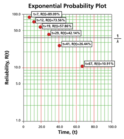
In order to plot the points for the probability plot, the appropriate reliability estimate values must be obtained. These will be equivalent to [math]\displaystyle{ 100%-MR\,\! }[/math] since the y-axis represents the reliability and the [math]\displaystyle{ MR\,\! }[/math] values represent unreliability estimates.
Next, these points are plotted on an exponential probability plotting paper. A sample of this type of plotting paper is shown next, with the sample points in place. Notice how these points describe a line with a negative slope.
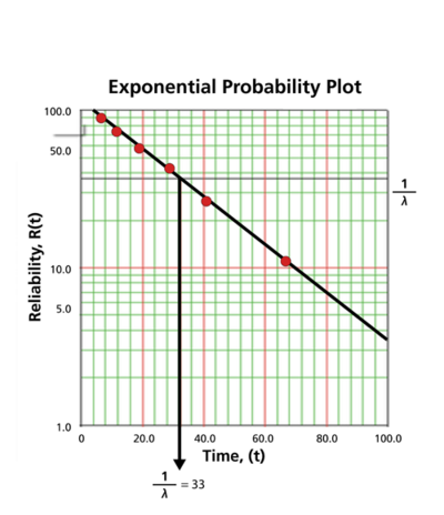
Once the points are plotted, draw the best possible straight line through these points. The time value at which this line intersects with a horizontal line drawn at the 36.8% reliability mark is the mean life, and the reciprocal of this is the failure rate [math]\displaystyle{ \lambda\,\! }[/math]. This is because at [math]\displaystyle{ t=m=\tfrac{1}{\lambda }\,\! }[/math]:
- [math]\displaystyle{ \begin{align} R(t)= & {{e}^{-\lambda \cdot t}} \\ R(t)= & {{e}^{-\lambda \cdot \tfrac{1}{\lambda }}} \\ R(t)= & {{e}^{-1}}=0.368=36.8%. \end{align}\,\! }[/math]
The following plot shows that the best-fit line through the data points crosses the [math]\displaystyle{ R=36.8%\,\! }[/math] line at [math]\displaystyle{ t=33\,\! }[/math] hours. And because [math]\displaystyle{ \tfrac{1}{\lambda }=33\,\! }[/math] hours, [math]\displaystyle{ \lambda =0.0303\,\! }[/math] failures/hour.
The exponential distribution is a commonly used distribution in reliability engineering. Mathematically, it is a fairly simple distribution, which many times leads to its use in inappropriate situations. It is, in fact, a special case of the Weibull distribution where [math]\displaystyle{ \beta =1\,\! }[/math]. The exponential distribution is used to model the behavior of units that have a constant failure rate (or units that do not degrade with time or wear out).
Exponential Probability Density Function
The 2-Parameter Exponential Distribution
The 2-parameter exponential pdf is given by:
- [math]\displaystyle{ f(t)=\lambda {{e}^{-\lambda (t-\gamma )}},f(t)\ge 0,\lambda \gt 0,t\ge \gamma \,\! }[/math]
where [math]\displaystyle{ \gamma \,\! }[/math] is the location parameter. Some of the characteristics of the 2-parameter exponential distribution are discussed in Kececioglu [19]:
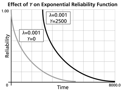
- The location parameter, [math]\displaystyle{ \gamma \,\! }[/math], if positive, shifts the beginning of the distribution by a distance of [math]\displaystyle{ \gamma \,\! }[/math] to the right of the origin, signifying that the chance failures start to occur only after [math]\displaystyle{ \gamma \,\! }[/math] hours of operation, and cannot occur before.
- The scale parameter is [math]\displaystyle{ \tfrac{1}{\lambda }=\bar{t}-\gamma =m-\gamma \,\! }[/math].
- The exponential pdf has no shape parameter, as it has only one shape.
- The distribution starts at [math]\displaystyle{ t=\gamma \,\! }[/math] at the level of [math]\displaystyle{ f(t=\gamma )=\lambda \,\! }[/math] and decreases thereafter exponentially and monotonically as [math]\displaystyle{ t\,\! }[/math] increases beyond [math]\displaystyle{ \gamma \,\! }[/math] and is convex.
- As [math]\displaystyle{ t\to \infty \,\! }[/math], [math]\displaystyle{ f(t)\to 0\,\! }[/math].
The 1-Parameter Exponential Distribution
The 1-parameter exponential pdf is obtained by setting [math]\displaystyle{ \gamma =0\,\! }[/math], and is given by:
- [math]\displaystyle{ \begin{align}f(t)= & \lambda {{e}^{-\lambda t}}=\frac{1}{m}{{e}^{-\tfrac{1}{m}t}}, & t\ge 0, \lambda \gt 0,m\gt 0 \end{align} \,\! }[/math]
where:
- [math]\displaystyle{ \lambda \,\! }[/math] = constant rate, in failures per unit of measurement, (e.g., failures per hour, per cycle, etc.)
- [math]\displaystyle{ \lambda =\frac{1}{m}\,\! }[/math]
- [math]\displaystyle{ m\,\! }[/math] = mean time between failures, or to failure
- [math]\displaystyle{ t\,\! }[/math] = operating time, life, or age, in hours, cycles, miles, actuations, etc.
This distribution requires the knowledge of only one parameter, [math]\displaystyle{ \lambda \,\! }[/math], for its application. Some of the characteristics of the 1-parameter exponential distribution are discussed in Kececioglu [19]:
- The location parameter, [math]\displaystyle{ \gamma \,\! }[/math], is zero.
- The scale parameter is [math]\displaystyle{ \tfrac{1}{\lambda }=m\,\! }[/math].
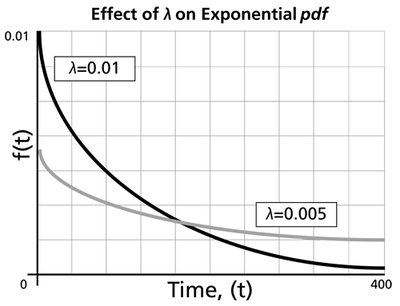
- As [math]\displaystyle{ \lambda \,\! }[/math] is decreased in value, the distribution is stretched out to the right, and as [math]\displaystyle{ \lambda \,\! }[/math] is increased, the distribution is pushed toward the origin.
- This distribution has no shape parameter as it has only one shape, (i.e., the exponential, and the only parameter it has is the failure rate, [math]\displaystyle{ \lambda \,\! }[/math]).
- The distribution starts at [math]\displaystyle{ t=0\,\! }[/math] at the level of [math]\displaystyle{ f(t=0)=\lambda \,\! }[/math] and decreases thereafter exponentially and monotonically as [math]\displaystyle{ t\,\! }[/math] increases, and is convex.
- As [math]\displaystyle{ t\to \infty \,\! }[/math], [math]\displaystyle{ f(t)\to 0\,\! }[/math].
- The pdf can be thought of as a special case of the Weibull pdf with [math]\displaystyle{ \gamma =0\,\! }[/math] and [math]\displaystyle{ \beta =1\,\! }[/math].
Exponential Distribution Functions
The Mean or MTTF
The mean, [math]\displaystyle{ \overline{T},\,\! }[/math] or mean time to failure (MTTF) is given by:
- [math]\displaystyle{ \begin{align} \bar{T}= & \int_{\gamma }^{\infty }t\cdot f(t)dt \\ = & \int_{\gamma }^{\infty }t\cdot \lambda \cdot {{e}^{-\lambda t}}dt \\ = & \gamma +\frac{1}{\lambda }=m \end{align}\,\! }[/math]
Note that when [math]\displaystyle{ \gamma =0\,\! }[/math], the MTTF is the inverse of the exponential distribution's constant failure rate. This is only true for the exponential distribution. Most other distributions do not have a constant failure rate. Consequently, the inverse relationship between failure rate and MTTF does not hold for these other distributions.
The Median
The median, [math]\displaystyle{ \breve{T}, \,\! }[/math] is:
- [math]\displaystyle{ \breve{T}=\gamma +\frac{1}{\lambda}\cdot 0.693 \,\! }[/math]
The Mode
The mode, [math]\displaystyle{ \tilde{T},\,\! }[/math] is:
- [math]\displaystyle{ \tilde{T}=\gamma \,\! }[/math]
The Standard Deviation
The standard deviation, [math]\displaystyle{ {\sigma }_{T}\,\! }[/math], is:
- [math]\displaystyle{ {\sigma}_{T}=\frac{1}{\lambda }=m\,\! }[/math]
The Exponential Reliability Function
The equation for the 2-parameter exponential cumulative density function, or cdf, is given by:
- [math]\displaystyle{ \begin{align} F(t)=Q(t)=1-{{e}^{-\lambda (t-\gamma )}} \end{align}\,\! }[/math]
Recalling that the reliability function of a distribution is simply one minus the cdf, the reliability function of the 2-parameter exponential distribution is given by:
- [math]\displaystyle{ R(t)=1-Q(t)=1-\int_{0}^{t-\gamma }f(x)dx\,\! }[/math]
- [math]\displaystyle{ R(t)=1-\int_{0}^{t-\gamma }\lambda {{e}^{-\lambda x}}dx={{e}^{-\lambda (t-\gamma )}}\,\! }[/math]
The 1-parameter exponential reliability function is given by:
- [math]\displaystyle{ R(t)={{e}^{-\lambda t}}={{e}^{-\tfrac{t}{m}}}\,\! }[/math]
The Exponential Conditional Reliability Function
The exponential conditional reliability equation gives the reliability for a mission of [math]\displaystyle{ t\,\! }[/math] duration, having already successfully accumulated [math]\displaystyle{ T\,\! }[/math] hours of operation up to the start of this new mission. The exponential conditional reliability function is:
- [math]\displaystyle{ R(t|T)=\frac{R(T+t)}{R(T)}=\frac{{{e}^{-\lambda (T+t-\gamma )}}}{{{e}^{-\lambda (T-\gamma )}}}={{e}^{-\lambda t}}\,\! }[/math]
which says that the reliability for a mission of [math]\displaystyle{ t\,\! }[/math] duration undertaken after the component or equipment has already accumulated [math]\displaystyle{ T\,\! }[/math] hours of operation from age zero is only a function of the mission duration, and not a function of the age at the beginning of the mission. This is referred to as the memoryless property.
The Exponential Reliable Life Function
The reliable life, or the mission duration for a desired reliability goal, [math]\displaystyle{ {{t}_{R}}\,\! }[/math], for the 1-parameter exponential distribution is:
- [math]\displaystyle{ R({{t}_{R}})={{e}^{-\lambda ({{t}_{R}}-\gamma )}}\,\! }[/math]
- [math]\displaystyle{ \begin{align} \ln[R({{t}_{R}})]=-\lambda({{t}_{R}}-\gamma ) \end{align}\,\! }[/math]
or:
- [math]\displaystyle{ {{t}_{R}}=\gamma -\frac{\ln [R({{t}_{R}})]}{\lambda }\,\! }[/math]
The Exponential Failure Rate Function
The exponential failure rate function is:
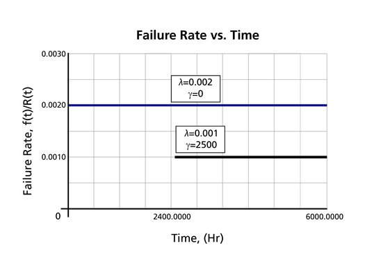
- [math]\displaystyle{ \lambda (t)=\frac{f(t)}{R(t)}=\frac{\lambda {{e}^{-\lambda (t-\gamma )}}}{{{e}^{-\lambda (t-\gamma )}}}=\lambda =\text{constant}\,\! }[/math]
Once again, note that the constant failure rate is a characteristic of the exponential distribution, and special cases of other distributions only. Most other distributions have failure rates that are functions of time.
Characteristics of the Exponential Distribution
The primary trait of the exponential distribution is that it is used for modeling the behavior of items with a constant failure rate. It has a fairly simple mathematical form, which makes it fairly easy to manipulate. Unfortunately, this fact also leads to the use of this model in situations where it is not appropriate. For example, it would not be appropriate to use the exponential distribution to model the reliability of an automobile. The constant failure rate of the exponential distribution would require the assumption that the automobile would be just as likely to experience a breakdown during the first mile as it would during the one-hundred-thousandth mile. Clearly, this is not a valid assumption. However, some inexperienced practitioners of reliability engineering and life data analysis will overlook this fact, lured by the siren-call of the exponential distribution's relatively simple mathematical models.
The Effect of lambda and gamma on the Exponential pdf
- The exponential pdf has no shape parameter, as it has only one shape.
- The exponential pdf is always convex and is stretched to the right as [math]\displaystyle{ \lambda \,\! }[/math] decreases in value.
- The value of the pdf function is always equal to the value of [math]\displaystyle{ \lambda \,\! }[/math] at [math]\displaystyle{ t=0\,\! }[/math] (or [math]\displaystyle{ t=\gamma \,\! }[/math]).
- The location parameter, [math]\displaystyle{ \gamma \,\! }[/math], if positive, shifts the beginning of the distribution by a distance of [math]\displaystyle{ \gamma \,\! }[/math] to the right of the origin, signifying that the chance failures start to occur only after [math]\displaystyle{ \gamma \,\! }[/math] hours of operation, and cannot occur before this time.
- The scale parameter is [math]\displaystyle{ \tfrac{1}{\lambda }=\bar{T}-\gamma =m-\gamma \,\! }[/math].
- As [math]\displaystyle{ t\to \infty \,\! }[/math], [math]\displaystyle{ f(t)\to 0\,\! }[/math].
The Effect of lambda and gamma on the Exponential Reliability Function
- The 1-parameter exponential reliability function starts at the value of 100% at [math]\displaystyle{ t=0\,\! }[/math], decreases thereafter monotonically and is convex.
- The 2-parameter exponential reliability function remains at the value of 100% for [math]\displaystyle{ t=0\,\! }[/math] up to [math]\displaystyle{ t=\gamma \,\! }[/math], and decreases thereafter monotonically and is convex.
- As [math]\displaystyle{ t\to \infty \,\! }[/math], [math]\displaystyle{ R(t\to \infty )\to 0\,\! }[/math].
- The reliability for a mission duration of [math]\displaystyle{ t=m=\tfrac{1}{\lambda }\,\! }[/math], or of one MTTF duration, is always equal to [math]\displaystyle{ 0.3679\,\! }[/math] or 36.79%. This means that the reliability for a mission which is as long as one MTTF is relatively low and is not recommended because only 36.8% of the missions will be completed successfully. In other words, of the equipment undertaking such a mission, only 36.8% will survive their mission.
The Effect of lambda and gamma on the Failure Rate Function
- The 1-parameter exponential failure rate function is constant and starts at [math]\displaystyle{ t=0\,\! }[/math].
- The 2-parameter exponential failure rate function remains at the value of 0 for [math]\displaystyle{ t=0\,\! }[/math] up to [math]\displaystyle{ t=\gamma \,\! }[/math], and then keeps at the constant value of [math]\displaystyle{ \lambda\,\! }[/math].
Exponential Distribution Examples
Grouped Data
20 units were reliability tested with the following results:
| Table - Life Test Data | |
| Number of Units in Group | Time-to-Failure |
|---|---|
| 7 | 100 |
| 5 | 200 |
| 3 | 300 |
| 2 | 400 |
| 1 | 500 |
| 2 | 600 |
1. Assuming a 2-parameter exponential distribution, estimate the parameters by hand using the MLE analysis method.
2. Repeat the above using Weibull++. (Enter the data as grouped data to duplicate the results.)
3. Show the Probability plot for the analysis results.
4. Show the Reliability vs. Time plot for the results.
5. Show the pdf plot for the results.
6. Show the Failure Rate vs. Time plot for the results.
7. Estimate the parameters using the rank regression on Y (RRY) analysis method (and using grouped ranks).
Solution
1. For the 2-parameter exponential distribution and for [math]\displaystyle{ \hat{\gamma }=100\,\! }[/math] hours (first failure), the partial of the log-likelihood function, [math]\displaystyle{ \lambda\,\! }[/math], becomes:
- [math]\displaystyle{ \begin{align} \frac{\partial \Lambda }{\partial \lambda }= &\underset{i=1}{\overset{6}{\mathop \sum }}\,{N_i} \left[ \frac{1}{\lambda }-\left( {{T}_{i}}-100 \right) \right]=0\\ \Rightarrow & 7[\frac{1}{\lambda }-(100-100)]+5[\frac{1}{\lambda}-(200-100)] + \ldots +2[\frac{1}{\lambda}-(600-100)]\\ = & 0\\ \Rightarrow & \hat{\lambda}=\frac{20}{3100}=0.0065 \text{fr/hr} \end{align} \,\! }[/math]
2. Enter the data in a Weibull++ standard folio and calculate it as shown next.
3. On the Plot page of the folio, the exponential Probability plot will appear as shown next.
4. View the Reliability vs. Time plot.
5. View the pdf plot.
6. View the Failure Rate vs. Time plot.
Note that, as described at the beginning of this chapter, the failure rate for the exponential distribution is constant. Also note that the Failure Rate vs. Time plot does show values for times before the location parameter, [math]\displaystyle{ \gamma \,\! }[/math], at 100 hours.
7. In the case of grouped data, one must be cautious when estimating the parameters using a rank regression method. This is because the median rank values are determined from the total number of failures observed by time [math]\displaystyle{ {{T}_{i}}\,\! }[/math] where [math]\displaystyle{ i\,\! }[/math] indicates the group number. In this example, the total number of groups is [math]\displaystyle{ N=6\,\! }[/math] and the total number of units is [math]\displaystyle{ {{N}_{T}}=20\,\! }[/math]. Thus, the median rank values will be estimated for 20 units and for the total failed units ([math]\displaystyle{ {{N}_{{{F}_{i}}}}\,\! }[/math]) up to the [math]\displaystyle{ {{i}^{th}}\,\! }[/math] group, for the [math]\displaystyle{ {{i}^{th}}\,\! }[/math] rank value. The median ranks values can be found from rank tables or they can be estimated using ReliaSoft's Quick Statistical Reference tool.
For example, the median rank value of the fourth group will be the [math]\displaystyle{ {{17}^{th}}\,\! }[/math] rank out of a sample size of twenty units (or 81.945%).
The following table is then constructed.
Given the values in the table above, calculate [math]\displaystyle{ \hat{a}\,\! }[/math] and [math]\displaystyle{ \hat{b}\,\! }[/math]:
- [math]\displaystyle{ \begin{align} & \hat{b}= & \frac{\underset{i=1}{\overset{6}{\mathop{\sum }}}\,{{t}_{i}}{{y}_{i}}-(\underset{i=1}{\overset{6}{\mathop{\sum }}}\,{{t}_{i}})(\underset{i=1}{\overset{6}{\mathop{\sum }}}\,{{y}_{i}})/6}{\underset{i=1}{\overset{6}{\mathop{\sum }}}\,t_{i}^{2}-{{(\underset{i=1}{\overset{6}{\mathop{\sum }}}\,{{t}_{i}})}^{2}}/6} \\ & & \\ & \hat{b}= & \frac{-4320.3362-(2100)(-9.6476)/6}{910,000-{{(2100)}^{2}}/6} \end{align}\,\! }[/math]
or:
- [math]\displaystyle{ \hat{b}=-0.005392\,\! }[/math]
and:
- [math]\displaystyle{ \hat{a}=\overline{y}-\hat{b}\overline{t}=\frac{\underset{i=1}{\overset{N}{\mathop{\sum }}}\,{{y}_{i}}}{N}-\hat{b}\frac{\underset{i=1}{\overset{N}{\mathop{\sum }}}\,{{t}_{i}}}{N}\,\! }[/math]
or:
- [math]\displaystyle{ \hat{a}=\frac{-9.6476}{6}-(-0.005392)\frac{2100}{6}=0.2793\,\! }[/math]
Therefore:
- [math]\displaystyle{ \hat{\lambda }=-\hat{b}=-(-0.005392)=0.05392\text{ failures/hour}\,\! }[/math]
and:
- [math]\displaystyle{ \hat{\gamma }=\frac{\hat{a}}{\hat{\lambda }}=\frac{0.2793}{0.005392}\,\! }[/math]
or:
- [math]\displaystyle{ \hat{\gamma }\simeq 51.8\text{ hours}\,\! }[/math]
Then:
- [math]\displaystyle{ f(T)=(0.005392){{e}^{-0.005392(T-51.8)}}\,\! }[/math]
Using Weibull++, the estimated parameters are:
- [math]\displaystyle{ \begin{align} \hat{\lambda }= & 0.0054\text{ failures/hour} \\ \hat{\gamma }= & 51.82\text{ hours} \end{align}\,\! }[/math]
The small difference in the values from Weibull++ is due to rounding. In the application, the calculations and the rank values are carried out up to the [math]\displaystyle{ 15^{th}\,\! }[/math] decimal point.
Using Auto Batch Run
A number of leukemia patients were treated with either drug 6MP or a placebo, and the times in weeks until cancer symptoms returned were recorded. Analyze each treatment separately [21, p.175].
| Table - Leukemia Treatment Results | |||
| Time (weeks) | Number of Patients | Treament | Comments |
|---|---|---|---|
| 1 | 2 | placebo | |
| 2 | 2 | placebo | |
| 3 | 1 | placebo | |
| 4 | 2 | placebo | |
| 5 | 2 | placebo | |
| 6 | 4 | 6MP | 3 patients completed |
| 7 | 1 | 6MP | |
| 8 | 4 | placebo | |
| 9 | 1 | 6MP | Not completed |
| 10 | 2 | 6MP | 1 patient completed |
| 11 | 2 | placebo | |
| 11 | 1 | 6MP | Not completed |
| 12 | 2 | placebo | |
| 13 | 1 | 6MP | |
| 15 | 1 | placebo | |
| 16 | 1 | 6MP | |
| 17 | 1 | placebo | |
| 17 | 1 | 6MP | Not completed |
| 19 | 1 | 6MP | Not completed |
| 20 | 1 | 6MP | Not completed |
| 22 | 1 | placebo | |
| 22 | 1 | 6MP | |
| 23 | 1 | placebo | |
| 23 | 1 | 6MP | |
| 25 | 1 | 6MP | Not completed |
| 32 | 2 | 6MP | Not completed |
| 34 | 1 | 6MP | Not completed |
| 35 | 1 | 6MP | Not completed |
Create a new Weibull++ standard folio that's configured for grouped times-to-failure data with suspensions. In the first column, enter the number of patients. Whenever there are uncompleted tests, enter the number of patients who completed the test separately from the number of patients who did not (e.g., if 4 patients had symptoms return after 6 weeks and only 3 of them completed the test, then enter 1 in one row and 3 in another). In the second column enter F if the patients completed the test and S if they didn't. In the third column enter the time, and in the fourth column (Subset ID) specify whether the 6MP drug or a placebo was used.
Next, open the Batch Auto Run utility and select to separate the 6MP drug from the placebo, as shown next.
The software will create two data sheets, one for each subset ID, as shown next.
Calculate both data sheets using the 2-parameter exponential distribution and the MLE analysis method, then insert an additional plot and select to show the analysis results for both data sheets on that plot, which will appear as shown next.
The normal distribution, also known as the Gaussian distribution, is the most widely-used general purpose distribution. It is for this reason that it is included among the lifetime distributions commonly used for reliability and life data analysis. There are some who argue that the normal distribution is inappropriate for modeling lifetime data because the left-hand limit of the distribution extends to negative infinity. This could conceivably result in modeling negative times-to-failure. However, provided that the distribution in question has a relatively high mean and a relatively small standard deviation, the issue of negative failure times should not present itself as a problem. Nevertheless, the normal distribution has been shown to be useful for modeling the lifetimes of consumable items, such as printer toner cartridges.
Normal Probability Density Function
The pdf of the normal distribution is given by:
- [math]\displaystyle{ f(t)=\frac{1}{\sigma \sqrt{2\pi }}{{e}^{-\frac{1}{2}{{\left( \frac{t-\mu }{\sigma } \right)}^{2}}}}\,\! }[/math]
where:
- [math]\displaystyle{ \mu\,\! }[/math] = mean of the normal times-to-faiure, also noted as [math]\displaystyle{ \bar{T}\,\! }[/math],
- [math]\displaystyle{ \theta\,\! }[/math] = standard deviation of the times-to-failure
It is a 2-parameter distribution with parameters [math]\displaystyle{ \mu \,\! }[/math] (or [math]\displaystyle{ \bar{T}\,\! }[/math] ) and [math]\displaystyle{ {{\sigma }}\,\! }[/math] (i.e., the mean and the standard deviation, respectively).
Normal Statistical Properties
The Normal Mean, Median and Mode
The normal mean or MTTF is actually one of the parameters of the distribution, usually denoted as [math]\displaystyle{ \mu .\,\! }[/math] Because the normal distribution is symmetrical, the median and the mode are always equal to the mean:
- [math]\displaystyle{ \mu =\tilde{T}=\breve{T}\,\! }[/math]
The Normal Standard Deviation
As with the mean, the standard deviation for the normal distribution is actually one of the parameters, usually denoted as [math]\displaystyle{ {{\sigma }_{T}}\,\! }[/math].
The Normal Reliability Function
The reliability for a mission of time [math]\displaystyle{ T\,\! }[/math] for the normal distribution is determined by:
- [math]\displaystyle{ R(t)=\int_{t}^{\infty }f(x)dx=\int_{t}^{\infty }\frac{1}{{{\sigma }}\sqrt{2\pi }}{{e}^{-\tfrac{1}{2}{{\left( \tfrac{x-\mu }{{{\sigma }}} \right)}^{2}}}}dx\,\! }[/math]
There is no closed-form solution for the normal reliability function. Solutions can be obtained via the use of standard normal tables. Since the application automatically solves for the reliability, we will not discuss manual solution methods. For interested readers, full explanations can be found in the references.
The Normal Conditional Reliability Function
The normal conditional reliability function is given by:
- [math]\displaystyle{ R(t|T)=\frac{R(T+t)}{R(T)}=\frac{\int_{T+t}^{\infty }\tfrac{1}{{{\sigma }}\sqrt{2\pi }}{{e}^{-\tfrac{1}{2}{{\left( \tfrac{x-\mu }{{{\sigma }}} \right)}^{2}}}}dx}{\int_{T}^{\infty }\tfrac{1}{{{\sigma }}\sqrt{2\pi }}{{e}^{-\tfrac{1}{2}{{\left( \tfrac{x-\mu }{{{\sigma }}} \right)}^{2}}}}dx}\,\! }[/math]
Once again, the use of standard normal tables for the calculation of the normal conditional reliability is necessary, as there is no closed form solution.
The Normal Reliable Life
Since there is no closed-form solution for the normal reliability function, there will also be no closed-form solution for the normal reliable life. To determine the normal reliable life, one must solve:
- [math]\displaystyle{ R(T)=\int_{T}^{\infty }\frac{1}{{{\sigma }}\sqrt{2\pi }}{{e}^{-\tfrac{1}{2}{{\left( \tfrac{t-\mu }{{{\sigma }}} \right)}^{2}}}}dt\,\! }[/math]
for [math]\displaystyle{ T\,\! }[/math].
The Normal Failure Rate Function
The instantaneous normal failure rate is given by:
- [math]\displaystyle{ \lambda (t)=\frac{f(t)}{R(t)}=\frac{\tfrac{1}{{{\sigma }}\sqrt{2\pi }}{{e}^{-\tfrac{1}{2}{{\left( \tfrac{t-\mu }{{{\sigma }}} \right)}^{2}}}}}{\int_{t}^{\infty }\tfrac{1}{{{\sigma }}\sqrt{2\pi }}{{e}^{-\tfrac{1}{2}{{\left( \tfrac{x-\mu }{{{\sigma }}} \right)}^{2}}}}dx}\,\! }[/math]
Characteristics of the Normal Distribution
Some of the specific characteristics of the normal distribution are the following:
- The normal pdf has a mean, [math]\displaystyle{ \bar{T}\,\! }[/math], which is equal to the median, [math]\displaystyle{ \breve{T}\,\! }[/math], and also equal to the mode, [math]\displaystyle{ \tilde{T}\,\! }[/math], or [math]\displaystyle{ \bar{T}=\breve{T}=\tilde{T}\,\! }[/math]. This is because the normal distribution is symmetrical about its mean.
- The mean, [math]\displaystyle{ \mu \,\! }[/math], or the mean life or the [math]\displaystyle{ MTTF\,\! }[/math], is also the location parameter of the normal pdf, as it locates the pdf along the abscissa. It can assume values of [math]\displaystyle{ -\infty \lt \bar{T}\lt \infty \,\! }[/math].
- The normal pdf has no shape parameter. This means that the normal pdf has only one shape, the bell shape, and this shape does not change.
- The standard deviation, [math]\displaystyle{ {{\sigma }}\,\! }[/math], is the scale parameter of the normal pdf.
- As [math]\displaystyle{ {{\sigma }}\,\! }[/math] decreases, the pdf gets pushed toward the mean, or it becomes narrower and taller.
- As [math]\displaystyle{ {{\sigma }}\,\! }[/math] increases, the pdf spreads out away from the mean, or it becomes broader and shallower.
- The standard deviation can assume values of [math]\displaystyle{ 0\lt {{\sigma }}\lt \infty \,\! }[/math].
- The greater the variability, the larger the value of [math]\displaystyle{ {{\sigma }}\,\! }[/math], and vice versa.
- The standard deviation is also the distance between the mean and the point of inflection of the pdf, on each side of the mean. The point of inflection is that point of the pdf where the slope changes its value from a decreasing to an increasing one, or where the second derivative of the pdf has a value of zero.
- The normal pdf starts at [math]\displaystyle{ t=-\infty \,\! }[/math] with an [math]\displaystyle{ f(t)=0\,\! }[/math]. As [math]\displaystyle{ t\,\! }[/math] increases, [math]\displaystyle{ f(t)\,\! }[/math] also increases, goes through its point of inflection and reaches its maximum value at [math]\displaystyle{ t=\bar{T}\,\! }[/math]. Thereafter, [math]\displaystyle{ f(t)\,\! }[/math] decreases, goes through its point of inflection, and assumes a value of [math]\displaystyle{ f(t)=0\,\! }[/math] at [math]\displaystyle{ t=+\infty \,\! }[/math].
Weibull++ Notes on Negative Time Values
One of the disadvantages of using the normal distribution for reliability calculations is the fact that the normal distribution starts at negative infinity. This can result in negative values for some of the results. Negative values for time are not accepted in most of the components of Weibull++, nor are they implemented. Certain components of the application reserve negative values for suspensions, or will not return negative results. For example, the Quick Calculation Pad will return a null value (zero) if the result is negative. Only the Free-Form (Probit) data sheet can accept negative values for the random variable (x-axis values).
Normal Distribution Examples
The following examples illustrate the different types of life data that can be analyzed in Weibull++ using the normal distribution. For more information on the different types of life data, see Life Data Classification.
Complete Data Example
6 units are tested to failure. The following failure times data are obtained: 12125, 11260, 12080, 12825, 13550 and 14670 hours. Assuming that the data are normally distributed, do the following:
Objectives
- 1. Find the parameters for the data set, using the Rank Regression on X (RRX) parameter estimation method
- 2. Obtain the probability plot for the data with 90%, two-sided Type 1 confidence bounds.
- 3. Obtain the pdf plot for the data.
- 4. Using the Quick Calculation Pad (QCP), determine the reliability for a mission of 11,000 hours, as well as the upper and lower two-sided 90% confidence limit on this reliability.
- 5. Using the QCP, determine the MTTF, as well as the upper and lower two-sided 90% confidence limit on this MTTF.
- 6. Obtain tabulated values for the failure rate for 10 different mission end times. The mission end times are 1,000 to 10,000 hours, using increments of 1,000 hours.
Solution
The following figure shows the data as entered in Weibull++, as well as the calculated parameters.
The following figures show the probability plot with the 90% two-sided confidence bounds and the pdf plot.
Both the reliability and MTTF can be easily obtained from the QCP. The QCP, with results, for both cases is shown in the next two figures.
To obtain tabulated values for the failure rate, use the Analysis Workbook or General Spreadsheet features that are included in Weibull++. (For more information on these features, please refer to the Weibull++ User's Guide. For a step-by-step example on creating Weibull++ reports, please see the Quick Start Guide). The following worksheet shows the mission times and the corresponding failure rates.
Suspension Data Example
19 units are being reliability tested and the following is a table of their times-to-failure and suspensions.
| Non-Grouped Data Times-to-Failure Data with Suspensions | ||
| Data point index | Last Inspected | State End Time |
|---|---|---|
| 1 | F | 2 |
| 2 | S | 3 |
| 3 | F | 5 |
| 4 | S | 7 |
| 5 | F | 11 |
| 6 | S | 13 |
| 7 | S | 17 |
| 8 | S | 19 |
| 9 | F | 23 |
| 10 | F | 29 |
| 11 | S | 31 |
| 12 | F | 37 |
| 13 | S | 41 |
| 14 | F | 43 |
| 15 | S | 47 |
| 16 | S | 53 |
| 17 | F | 59 |
| 18 | S | 61 |
| 19 | S | 67 |
Using the normal distribution and the maximum likelihood (MLE) parameter estimation method, the computed parameters are:
- [math]\displaystyle{ \begin{align} & \widehat{\mu }= & 48.07 \\ & {{{\hat{\sigma }}}_{T}}= & 28.41. \end{align}\,\! }[/math]
If we analyze the data set with the rank regression on x (RRX) method, the computed parameters are:
- [math]\displaystyle{ \begin{align} & \widehat{\mu }= & 46.40 \\ & {{{\hat{\sigma }}}_{T}}= & 28.64. \end{align}\,\! }[/math]
For the rank regression on y (RRY) method, the parameters are:
- [math]\displaystyle{ \begin{align} & \widehat{\mu }= & 47.34 \\ & {{{\hat{\sigma }}}_{T}}= & 29.96. \end{align}\,\! }[/math]
Interval Censored Data Example
8 units are being reliability tested, and the following is a table of their failure times:
| Non-Grouped Interval Data | ||
| Data point index | Last Inspected | State End Time |
|---|---|---|
| 1 | 30 | 32 |
| 2 | 32 | 35 |
| 3 | 35 | 37 |
| 4 | 37 | 40 |
| 5 | 42 | 42 |
| 6 | 45 | 45 |
| 7 | 50 | 50 |
| 8 | 55 | 55 |
This is a sequence of interval times-to-failure data. Using the normal distribution and the maximum likelihood (MLE) parameter estimation method, the computed parameters are:
- [math]\displaystyle{ \begin{align} & \widehat{\mu }= & 41.40 \\ & {{{\hat{\sigma }}}_{T}}= & 7.740. \end{align}\,\! }[/math]
For rank regression on x:
- [math]\displaystyle{ \begin{align} & \widehat{\mu }= & 41.40 \\ & {{{\hat{\sigma }}}_{T}}= & 9.03. \end{align}\,\! }[/math]
If we analyze the data set with the rank regression on y (RRY) parameter estimation method, the computed parameters are:
- [math]\displaystyle{ \begin{align} & \widehat{\mu }= & 41.39 \\ & {{{\hat{\sigma }}}_{T}}= & 9.25. \end{align}\,\! }[/math]
The following plot shows the results if the data were analyzed using the rank regression on X (RRX) method.
Mixed Data Types Example
Suppose our data set includes left and right censored, interval censored and complete data, as shown in the following table.
| Grouped Data Times-to-Failure with Suspensions and Intervals (Interval, Left and Right Censored) | ||||
|---|---|---|---|---|
| Data point index | Number in State | Last Inspection | State (S or F) | State End Time |
| 1 | 1 | 10 | F | 10 |
| 2 | 1 | 20 | S | 20 |
| 3 | 2 | 0 | F | 30 |
| 4 | 2 | 40 | F | 40 |
| 5 | 1 | 50 | F | 50 |
| 6 | 1 | 60 | S | 60 |
| 7 | 1 | 70 | F | 70 |
| 8 | 2 | 20 | F | 80 |
| 9 | 1 | 10 | F | 85 |
| 10 | 1 | 100 | F | 100 |
Using the normal distribution and the maximum likelihood (MLE) parameter estimation method, the computed parameters are:
- [math]\displaystyle{ \begin{align} & \widehat{\mu }= & 48.11 \\ & {{{\hat{\sigma }}}_{T}}= & 26.42 \end{align}\,\! }[/math]
If we analyze the data set with the rank regression on x (RRX) method, the computed parameters are:
- [math]\displaystyle{ \begin{align} & \widehat{\mu }= & 49.99 \\ & {{{\hat{\sigma }}}_{T}}= & 30.17 \end{align}\,\! }[/math]
For the rank regression on y (RRY) method, the parameters are:
- [math]\displaystyle{ \begin{align} & \widehat{\mu }= & 51.61 \\ & {{{\hat{\sigma }}}_{T}}= & 33.07 \end{align}\,\! }[/math]
Comparison of Analysis Methods
8 units are being reliability tested, and the following is a table of their failure times:
| Non-Grouped Times-to-Failure Data | ||
| Data point index | State F or S | State End Time |
|---|---|---|
| 1 | F | 2 |
| 2 | F | 5 |
| 3 | F | 11 |
| 4 | F | 23 |
| 5 | F | 29 |
| 6 | F | 37 |
| 7 | F | 43 |
| 8 | F | 59 |
Using the normal distribution and the maximum likelihood (MLE) parameter estimation method, the computed parameters are:
- [math]\displaystyle{ \begin{align} & \widehat{\mu }= & 26.13 \\ & {{{\hat{\sigma }}}_{T}}= & 18.57 \end{align}\,\! }[/math]
If we analyze the data set with the rank regression on x (RRX) method, the computed parameters are:
- [math]\displaystyle{ \begin{align} & \widehat{\mu }= & 26.13 \\ & {{{\hat{\sigma }}}_{T}}= & 21.64 \end{align}\,\! }[/math]
For the rank regression on y (RRY) method, the parameters are:
- [math]\displaystyle{ \begin{align} & \widehat{\mu }= & 26.13 \\ & {{{\hat{\sigma }}}_{T}}= & 22.28. \end{align}\,\! }[/math]
- REDIRECT Gamma Distribution Example
Template:Generalized gamma distribution example
- REDIRECT Logistic Distribution Example
- REDIRECT Loglogistic Distribution Example
Verify using Monte Carlo simulation that if [math]\displaystyle{ {{t}_{i}}\,\! }[/math] follows a Weibull distribution with [math]\displaystyle{ \beta \,\! }[/math] and [math]\displaystyle{ \eta \,\! }[/math], then the [math]\displaystyle{ Ln({{t}_{i}})\,\! }[/math] follows a Gumbel distribution with [math]\displaystyle{ \mu =\ln (\eta )\,\! }[/math] and [math]\displaystyle{ \sigma =1/\beta )\,\! }[/math].
Let us assume that [math]\displaystyle{ {{t}_{i}}\,\! }[/math] follows a Weibull distribution with [math]\displaystyle{ \beta =0.5\,\! }[/math] and [math]\displaystyle{ \eta =10000\,\! }[/math]. The Monte Carlo simulation tool in Weibull++ can be used to generate a set of random numbers that follow a Weibull distribution with the specified parameters. The following picture shows the Main tab of the Monte Carlo Data Generation utility.
On the Settings tab, set the number of points to 100 and click Generate. This creates a new data sheet in the folio that contains random time values [math]\displaystyle{ {{t}_{i}}\,\! }[/math].
Insert a new data sheet in the folio and enter the corresponding [math]\displaystyle{ Ln({{t}_{i}})\,\! }[/math] values of the time values generated by the Monte Carlo simulation. Delete any negative values, if there are any, because Weibull++ expects the time values to be positive. After obtaining the [math]\displaystyle{ Ln({{t}_{i}})\,\! }[/math] values, analyze the data sheet using the Gumbel distribution and the MLE parameter estimation method. The estimated parameters are (your results may vary due to the random numbers generated by simulation):
- [math]\displaystyle{ \begin{align} & \hat{\mu }= & 9.3816 \\ & \hat{\sigma }= & 1.9717 \end{align}\,\! }[/math]
Because [math]\displaystyle{ \ln (\eta )= 9.2103\,\! }[/math] ( [math]\displaystyle{ \simeq 9.3816\,\! }[/math] ) and [math]\displaystyle{ 1/\beta =2\,\! }[/math] [math]\displaystyle{ (\simeq 1.9717)\,\! }[/math], then this simulation verifies that [math]\displaystyle{ Ln({{t}_{i}})\,\! }[/math] follows a Gumbel distribution with [math]\displaystyle{ \mu =\ln (\eta )\,\! }[/math] and [math]\displaystyle{ \delta =1/\beta \,\! }[/math].
Note: This example illustrates a property of the Gumbel distribution; it is not meant to be a formal proof.

