Template:Failure mode management strategy rga

Failure Mode Management Strategy

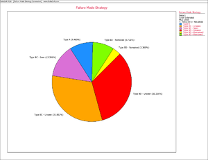
Management controls the resources for corrective actions. Consequently, the effectiveness factors are part of the management strategy. For the BD mode failure intensity that has been seen during development testing, 100 [math]\displaystyle{ d }[/math] percent will be removed and 100 [math]\displaystyle{ (1-d) }[/math] percent will remain in the system. Therefore, after the corrective actions have been made, the current system instantaneous failure intensity consists of the failure intensity due to the A modes plus the failure intensity for the unseen BC modes, plus the failure intensity for the unseen BD modes, plus the failure intensity for the BD modes that have been seen. Figure extendedpic4 shows how the system's instantaneous failure intensity can be broken down into its individual pieces based on the current failure mode strategy.

System failure intensity after the corrective actions.

Keep in mind that the individual components of the system's instantaneous failure intensity will depend on the classifications defined in the data. For example, if BC modes are not present within the data then the BC mode MTBF will not be a part of the overall system MTBF. The individual pieces of the pie, as shown Figure extendedpic4, are calculated using the following equations.

Let:

[math]\displaystyle{ \hat{r}(T)=\hat{\lambda }\hat{\beta }{{T}^{\hat{\beta }-1}} }[/math]

where [math]\displaystyle{ T }[/math] is the test time and [math]\displaystyle{ \hat{\beta } }[/math] and [math]\displaystyle{ \hat{\lambda } }[/math] are the maximum likelihood estimates of the Crow-AMSAA model for all of the data. [math]\displaystyle{ \hat{\beta } }[/math] is the biased estimate of [math]\displaystyle{ \beta }[/math] . Therefore:

[math]\displaystyle{ \hat{\beta }=\frac{N}{\underset{i=1}{\overset{N}{\mathop{\sum }}}\,\ln \left( \tfrac{T}{{{X}_{i}}} \right)} }[/math]

[math]\displaystyle{ \hat{\lambda }=\frac{N}{{{T}^{{\hat{\beta }}}}} }[/math]

where [math]\displaystyle{ N }[/math] is the total number of failures and [math]\displaystyle{ {{X}_{i}} }[/math] is the [math]\displaystyle{ {{i}^{th}} }[/math] time-to-failure. Let the successive failures [math]\displaystyle{ 0\lt {{X}_{1}}\lt {{X}_{2}}\lt \ldots \lt {{X}_{3}}\lt {{X}_{N}} }[/math] be partitioned into the A mode failures ( [math]\displaystyle{ {{N}_{A}} }[/math] ), BC first occurrence failures ( [math]\displaystyle{ {{N}_{BCF}} }[/math] ), BC remaining failures ( [math]\displaystyle{ {{N}_{BCR}} }[/math] ), BD first occurrence failure ( [math]\displaystyle{ {{N}_{BDF}} }[/math] ) and the BD remaining failures ( [math]\displaystyle{ {{N}_{BDR}} }[/math] ). For continuous data, each portion of the pie chart due to each of the modes is calculated as follows:

• A modes

[math]\displaystyle{ A=\left( \frac{T}{{{N}^{2}}} \right)\left[ \underset{i=1}{\overset{{{N}_{A}}}{\mathop \sum }}\,\ln \left( \frac{T}{{{X}_{Ai}}} \right) \right]\hat{r}(T) }[/math]

• BC modes unseen

[math]\displaystyle{ B{{C}_{unseen}}=\left( \frac{T}{{{N}^{2}}} \right)\left[ \underset{i=1}{\overset{{{N}_{BCF}}}{\mathop \sum }}\,\ln \left( \frac{T}{{{X}_{BCFi}}} \right) \right]\hat{r}(T) }[/math]

  • BC modes seen

[math]\displaystyle{ B{{C}_{seen}}=\left( \frac{T}{{{N}^{2}}} \right)\left[ \underset{i=1}{\overset{{{N}_{BCR}}}{\mathop \sum }}\,\ln \left( \frac{T}{{{X}_{BCRi}}} \right) \right]\hat{r}(T) }[/math]

• BD modes unseen

[math]\displaystyle{ B{{D}_{unseen}}=\left( \frac{T}{{{N}^{2}}} \right)\left[ \underset{i=1}{\overset{{{N}_{BDF}}}{\mathop \sum }}\,\ln \left( \frac{T}{{{X}_{BDFi}}} \right) \right]\hat{r}(T) }[/math]

• BD modes seen

[math]\displaystyle{ B{{D}_{seen}}=\left( \frac{T}{{{N}^{2}}} \right)\left[ \underset{i=1}{\overset{{{N}_{BDR}}}{\mathop \sum }}\,\ln \left( \frac{T}{{{X}_{BDRi}}} \right) \right]\hat{r}(T) }[/math]

• BD modes remain

[math]\displaystyle{ \begin{align} & B{{D}_{remain}}= & \left( 1-\frac{1}{M}\underset{i=1}{\overset{M}{\mathop \sum }}\,{{d}_{i}} \right)\cdot B{{D}_{seen}} \\ & = & \left( 1-\overline{d} \right)\cdot B{{D}_{seen}} \end{align} }[/math]

• BD modes removed

[math]\displaystyle{ \begin{align} & B{{D}_{removed}}= & \frac{1}{M}\underset{i=1}{\overset{M}{\mathop \sum }}\,{{d}_{i}}\cdot B{{D}_{seen}} \\ & = & \overline{d}\cdot B{{D}_{seen}} \end{align} }[/math]

For grouped data, from Chapter 5 the maximum likelihood estimates of [math]\displaystyle{ \beta }[/math] and [math]\displaystyle{ \lambda }[/math] are calculated such that the following equations are satisfied:

[math]\displaystyle{ \underset{i=1}{\overset{K}{\mathop \sum }}\,{{N}_{i}}\left[ \frac{t_{i}^{{\hat{\beta }}}\ln ({{t}_{i}})-t_{i-1}^{{\hat{\beta }}}\ln ({{t}_{i-1}})}{t_{i}^{{\hat{\beta }}}-t_{i-1}^{{\hat{\beta }}}}-\ln T \right]=0 }[/math]

[math]\displaystyle{ \hat{\lambda }=\frac{N}{T_{K}^{{\hat{\beta }}}} }[/math]

where [math]\displaystyle{ K }[/math] is the number of groups and [math]\displaystyle{ N=\underset{i=1}{\overset{K}{\mathop{\sum }}}\,{{N}_{i}} }[/math] .

• A modes

[math]\displaystyle{ A=\left( \frac{T}{{{N}^{2}}} \right)\left[ {{N}_{A}}\ln (T)-\underset{i=1}{\overset{K}{\mathop \sum }}\,\frac{{{N}_{Ai}}}{{\hat{\beta }}}\left( \frac{t_{i}^{{\hat{\beta }}}\ln (t_{i}^{{\hat{\beta }}})-t_{i-1}^{{\hat{\beta }}}\ln (t_{i-1}^{{\hat{\beta }}})}{t_{i}^{{\hat{\beta }}}-t_{i-1}^{{\hat{\beta }}}}-1 \right) \right]\hat{r}(T) }[/math]

• BC modes unseen

[math]\displaystyle{ B{{C}_{unseen}}=\left( \frac{T}{{{N}^{2}}} \right)\left[ {{N}_{BCF}}\ln (T)-\underset{i=1}{\overset{K}{\mathop \sum }}\,\frac{{{N}_{BCFi}}}{{\hat{\beta }}}\left( \frac{t_{i}^{{\hat{\beta }}}\ln (t_{i}^{{\hat{\beta }}})-t_{i-1}^{{\hat{\beta }}}\ln (t_{i-1}^{{\hat{\beta }}})}{t_{i}^{{\hat{\beta }}}-t_{i-1}^{{\hat{\beta }}}}-1 \right) \right]\hat{r}(T) }[/math]

• BC modes seen

[math]\displaystyle{ B{{C}_{seen}}=\left( \frac{T}{{{N}^{2}}} \right)\left[ {{N}_{BCR}}\ln (T)-\underset{i=1}{\overset{K}{\mathop \sum }}\,\frac{{{N}_{BCRi}}}{{\hat{\beta }}}\left( \frac{t_{i}^{{\hat{\beta }}}\ln (t_{i}^{{\hat{\beta }}})-t_{i-1}^{{\hat{\beta }}}\ln (t_{i-1}^{{\hat{\beta }}})}{t_{i}^{{\hat{\beta }}}-t_{i-1}^{{\hat{\beta }}}}-1 \right) \right]\hat{r}(T) }[/math]

• BD modes unseen

[math]\displaystyle{ B{{D}_{unseen}}=\left( \frac{T}{{{N}^{2}}} \right)\left[ {{N}_{BDF}}\ln (T)-\underset{i=1}{\overset{K}{\mathop \sum }}\,\frac{{{N}_{BDFi}}}{{\hat{\beta }}}\left( \frac{t_{i}^{{\hat{\beta }}}\ln (t_{i}^{{\hat{\beta }}})-t_{i-1}^{{\hat{\beta }}}\ln (t_{i-1}^{{\hat{\beta }}})}{t_{i}^{{\hat{\beta }}}-t_{i-1}^{{\hat{\beta }}}}-1 \right) \right]\hat{r}(T) }[/math]

• BD modes seen

[math]\displaystyle{ B{{D}_{seen}}=\left( \frac{T}{{{N}^{2}}} \right)\left[ {{N}_{BDR}}\ln (T)-\underset{i=1}{\overset{K}{\mathop \sum }}\,\frac{{{N}_{BDRi}}}{{\hat{\beta }}}\left( \frac{t_{i}^{{\hat{\beta }}}\ln (t_{i}^{{\hat{\beta }}})-t_{i-1}^{{\hat{\beta }}}\ln (t_{i-1}^{{\hat{\beta }}})}{t_{i}^{{\hat{\beta }}}-t_{i-1}^{{\hat{\beta }}}}-1 \right) \right]\hat{r}(T) }[/math]

  • BD modes remain

[math]\displaystyle{ \begin{align} & B{{D}_{remain}}= & \left( 1-\frac{1}{M}\underset{i=1}{\overset{M}{\mathop \sum }}\,{{d}_{i}} \right)\cdot B{{D}_{seen}} \\ & = & \left( 1-\overline{d} \right)\cdot B{{D}_{seen}} \end{align} }[/math]

• BD modes removed

[math]\displaystyle{ \begin{align} & B{{D}_{removed}}= & \frac{1}{M}\underset{i=1}{\overset{M}{\mathop \sum }}\,{{d}_{i}}\cdot B{{D}_{seen}} \\ & = & \overline{d}\cdot B{{D}_{seen}} \end{align} }[/math]

Example 2
Consider the data in Table 9.3. There were 56 total failures and [math]\displaystyle{ T=400 }[/math] . The effectiveness factors of the BD modes are given in Table 9.4. Determine the following:

1) Calculate the demonstrated MTBF and failure intensity.

2) Calculate the projected MTBF and failure intensity.

3) What is the rate at which unique BD modes are being generated during this test?

4) If the test continues for an additional 50 hours, what is the minimum number of new unique BD modes expected to be generated?

Table 9.3 - Test-fix-find-test data
[math]\displaystyle{ i }[/math]	[math]\displaystyle{ {{X}_{i}} }[/math]	Mode	[math]\displaystyle{ i }[/math]	[math]\displaystyle{ {{X}_{i}} }[/math]	Mode
1	0.7	BC17	29	192.7	BD11
2	3.7	BC17	30	213	A
3	13.2	BC17	31	244.8	A
4	15	BD1	32	249	BD12
5	17.6	BC18	33	250.8	A
6	25.3	BD2	34	260.1	BD1
7	47.5	BD3	35	263.5	BD8
8	54	BD4	36	273.1	A
9	54.5	BC19	37	274.7	BD6
10	56.4	BD5	38	282.8	BC27
11	63.6	A	39	285	BD13
12	72.2	BD5	40	304	BD9
13	99.2	BC20	41	315.4	BD4
14	99.6	BD6	42	317.1	A
15	100.3	BD7	43	320.6	A
16	102.5	A	44	324.5	BD12
17	112	BD8	45	324.9	BD10
18	112.2	BC21	46	342	BD5
19	120.9	BD2	47	350.2	BD3
20	121.9	BC22	48	355.2	BC28
21	125.5	BD9	49	364.6	BD10
22	133.4	BD10	50	364.9	A
23	151	BC23	51	366.3	BD2
24	163	BC24	52	373	BD8
25	164.7	BD9	53	379.4	BD14
26	174.5	BC25	54	389	BD15
27	177.4	BD10	55	394.9	A
28	191.6	BC26	56	395.2	BD16

Table 9.4 - Effectiveness factor for each unique BD mode
BD Mode	EF [math]\displaystyle{ {{d}_{i}} }[/math]
1	.67
2	.72
3	.77
4	.77
5	.87
6	.92
7	.50
8	.85
9	.89
10	.74
11	.70
12	.63
13	.64
14	.72
15	.69
16	.46

Solution

1) In order to obtain [math]\displaystyle{ {{\widehat{\lambda }}_{CA}} }[/math] , use the traditional Crow-AMSAA model for test-fix-test to fit all 56 data points, regardless of the failure mode classification to get:

[math]\displaystyle{ \begin{align} & \widehat{\beta }= & 0.91026 \\ & \widehat{\lambda }= & 0.23969 \end{align} }[/math]

Thus the achieved or demonstrated failure intensity is estimated by:

[math]\displaystyle{ \begin{align} & {{\widehat{\lambda }}_{CA}}= & \widehat{\lambda }\widehat{\beta }{{T}^{\widehat{\beta }-1}} \\ & = & 0.23969\times 0.91026\times {{400}^{(0.91026-1)}} \\ & = & 0.12744 \end{align} }[/math]

The achieved or demonstrated MTBF, [math]\displaystyle{ {{M}_{CA}} }[/math] , is the system reliability attained at the end of test, [math]\displaystyle{ T=400 }[/math] , and is estimated by:

[math]\displaystyle{ {{\widehat{M}}_{CA}}={{[{{\widehat{\lambda }}_{CA}}]}^{-1}}=7.84708 }[/math]

2) For this data set, [math]\displaystyle{ M=16 }[/math] and [math]\displaystyle{ T=400 }[/math] .

[math]\displaystyle{ {{\widehat{\lambda }}_{BD}}=\frac{{{N}_{BD}}}{T}=\frac{32}{400}=0.08 }[/math]

[math]\displaystyle{ \overline{d}=\underset{i=1}{\overset{M}{\mathop \sum }}\,{{d}_{i}}/M=0.72125 }[/math]

[math]\displaystyle{ \underset{i=1}{\overset{16}{\mathop \sum }}\,(1-{{d}_{i}}){{N}_{i}}/T=0.01955 }[/math]

Calculate [math]\displaystyle{ \hat{\beta } }[/math] and [math]\displaystyle{ \hat{\lambda } }[/math] of the BD modes using Eqns. (Extend1) and (Extend2):

[math]\displaystyle{ \begin{align} & {{{\hat{\beta }}}_{BD}}= & 0.74715 \\ & {{{\hat{\lambda }}}_{BD}}= & 0.18197 \end{align} }[/math]

Then:

[math]\displaystyle{ \overline{d}\widehat{h}(T|BD)=0.0215 }[/math]

Therefore:

[math]\displaystyle{ \begin{align} 43) & {{\widehat{\lambda }}_{EM}}= & {{\widehat{\lambda }}_{CA}}-{{\widehat{\lambda }}_{BD}}+\underset{i=1}{\overset{K}{\mathop \sum }}\,(1-{{d}_{i}})\frac{{{N}_{i}}}{T}+\overline{d}\widehat{h}(T|BD) \\ & = & 0.12744-0.08+0.0196+0.0215 \\ & = & 0.08854 \end{align} }[/math]

The Crow Extended model projected MTBF is:

[math]\displaystyle{ \begin{align} & {{\widehat{M}}_{EM}}= & {{[{{\widehat{\lambda }}_{EM}}]}^{-1}} \\ & = & 11.29418 \end{align} }[/math]

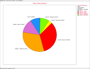
Consequently, based on the Crow Extended model and the data in Tables 9.3 and 9.4, the MTBF grew to 7.85 as a result of the corrective actions for the BC failure modes during the test. The MTBF then jumped to 11.29 after the test as a result of the delayed corrective actions for the BD failure modes. The management strategy can be summarized by the Failure Mode Strategy plot shown in Figure extendedpic5.

Figure extendedpic5 shows that 9.48% of the system's failure intensity has been left in (A modes), 31.81% of the failure intensity due to the BC modes has not been seen yet and 13.40% was removed during the test (BC modes - seen). In addition, 33.23% of the failure intensity due to the BD modes has not been seen yet, 3.37% will remain in the system since the corrective actions will not be completely effective at eliminating the identified failure modes and 8.72% will be removed after the delayed corrective actions.

3) The rate at which unique BD modes are being generated is equal to [math]\displaystyle{ h{{(T|BD)}^{-1}} }[/math] , where:

[math]\displaystyle{ \begin{align} & h{{(T|BD)}^{-1}}= & \frac{1}{{{\widehat{\lambda }}_{BD}}{{\widehat{\beta }}_{BD}}{{T}^{{{\widehat{\beta }}_{BD}}-1}}} \\ & = & \frac{T}{M{{\widehat{\beta }}_{BD}}} \\ & = & 33.4605 \end{align} }[/math]

4) Unique BD modes are being generated every 33.4605 hours. If the test continues for another 50 hours, then at least one new unique BD mode would be expected to be seen from this additional testing.

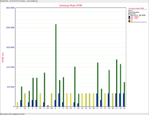
As shown in Figure extendedpic6, the MTBF of each individual failure mode can be plotted and the failure modes with the lowest MTBF can be identified. These are the failure modes that cause the majority of the system failures.

Failure Mode Strategy plot.

Individual Mode MTBF chart.