Template:Bounds on cumulative number of failures camsaa-gd
Bounds on Cumulative Number of Failures
Fisher Matrix Bounds
The cumulative number of failures, [math]\displaystyle{ N(t) }[/math] , must be positive, thus [math]\displaystyle{ \ln N(t) }[/math] is treated as being normally distributed.
- [math]\displaystyle{ \frac{\ln \hat{N}(t)-\ln N(t)}{\sqrt{Var(\ln \hat{N}(t)})}\ \tilde{\ }\ N(0,1) }[/math]
- [math]\displaystyle{ N(t)=\hat{N}(t){{e}^{\pm {{z}_{\alpha }}\sqrt{Var(\hat{N}(t))}/\hat{N}(t)}} }[/math]
- where:
- [math]\displaystyle{ \hat{N}(t)=\hat{\lambda }{{t}^{{\hat{\beta }}}} }[/math]
- [math]\displaystyle{ \begin{align} & Var(\hat{N}(t))= & {{\left( \frac{\partial \hat{N}(t)}{\partial \beta } \right)}^{2}}Var(\hat{\beta })+{{\left( \frac{\partial \hat{N}(t)}{\partial \lambda } \right)}^{2}}Var(\hat{\lambda }) \\ & & +2\left( \frac{\partial \hat{N}(t)}{\partial \beta } \right)\left( \frac{\partial \hat{N}(t)}{\partial \lambda } \right)cov(\hat{\beta },\hat{\lambda }) \end{align} }[/math]
The variance calculation is the same as Eqn. (variances) and:
- [math]\displaystyle{ \begin{align} & \frac{\partial \hat{N}(t)}{\partial \beta }= & \hat{\lambda }{{t}^{{\hat{\beta }}}}\ln t \\ & \frac{\partial \hat{N}(t)}{\partial \lambda }= & {{t}^{{\hat{\beta }}}} \end{align} }[/math]
Crow Bounds
The Crow confidence bounds on cumulative number of failures are:
- [math]\displaystyle{ \begin{align} & {{N}_{L}}(T)= & \frac{T}{{\hat{\beta }}}{{\lambda }_{i}}{{(T)}_{L}} \\ & {{N}_{U}}(T)= & \frac{T}{{\hat{\beta }}}{{\lambda }_{i}}{{(T)}_{U}} \end{align} }[/math]
where [math]\displaystyle{ {{\lambda }_{i}}{{(T)}_{L}} }[/math] and [math]\displaystyle{ {{\lambda }_{i}}{{(T)}_{U}} }[/math] can be obtained from Eqn. (dsaf).
Example 5
A new helicopter system is under development. System failure data has been collected on five helicopters during the final test phase. The actual failure times cannot be determined since the failures are not discovered until after the helicopters are brought into the maintenance area. However, total flying hours are known when the helicopters are brought in for service and every two weeks, each helicopter undergoes a thorough inspection to uncover any failures that may have occurred since the last inspection. Therefore, the cumulative total number of flight hours and the cumulative total number of failures for the five helicopters are known for each two-week period. The total number of flight hours from the test phase is 500, which was accrued over a period of 12 weeks (6 2-week intervals). For each 2-week interval, the total number of flight hours and total number of failures for the five helicopters were recorded. The grouped data set is displayed in Table 5.3.
| Interval | Interval Length | Failures in Interval |
|---|---|---|
| 1 | 0 - 62 | 12 |
| 2 | 62 -100 | 6 |
| 3 | 100 - 187 | 15 |
| 4 | 187 - 210 | 3 |
| 5 | 210 - 350 | 18 |
| 6 | 350 - 500 | 16 |
- 1) Estimate the parameters of the Crow-AMSAA model using maximum likelihood estimation.
- 2) Calculate the confidence bounds on the cumulative and instantaneous MTBF using the
Fisher Matrix and Crow methods.
Solution
- 1) Obtain the estimator of [math]\displaystyle{ \beta }[/math] using Eqn. (vv). Using RGA, the value of [math]\displaystyle{ \widehat{\beta } }[/math] is 0.81361. Now plug this value into Eqn. (vv1) and [math]\displaystyle{ \widehat{\lambda } }[/math] is:
- [math]\displaystyle{ \widehat{\lambda }=0.44585 }[/math]
Fisher Matrix confidence bounds can be obtained on the parameters [math]\displaystyle{ \widehat{\beta } }[/math] and [math]\displaystyle{ \widehat{\lambda } }[/math] at the 90% confidence level by:
- [math]\displaystyle{ \begin{align} & {{\beta }_{L}}= & \hat{\beta }{{e}^{{{z}_{\alpha }}\sqrt{Var(\hat{\beta })}/\hat{\beta }}} \\ & = & 0.6546 \\ & {{\beta }_{U}}= & \hat{\beta }{{e}^{-{{z}_{\alpha }}\sqrt{Var(\hat{\beta })}/\hat{\beta }}} \\ & = & 1.0112 \end{align} }[/math]
- and:
- [math]\displaystyle{ \begin{align} & {{\lambda }_{L}}= & \hat{\lambda }{{e}^{{{z}_{\alpha }}\sqrt{Var(\hat{\lambda })}/\hat{\lambda }}} \\ & = & 0.14594 \\ & {{\lambda }_{U}}= & \hat{\lambda }{{e}^{-{{z}_{\alpha }}\sqrt{Var(\hat{\lambda })}/\hat{\lambda }}} \\ & = & 1.36207 \end{align} }[/math]
Crow confidence bounds can also be obtained on the parameters [math]\displaystyle{ \widehat{\beta } }[/math] and [math]\displaystyle{ \widehat{\lambda } }[/math] at the 90% confidence level, as:
- [math]\displaystyle{ \begin{align} & {{\beta }_{L}}= & \hat{\beta }(1-S) \\ & = & 0.63552 \\ & {{\beta }_{U}}= & \hat{\beta }(1+S) \\ & = & 0.99170 \end{align} }[/math]
- and:
- [math]\displaystyle{ \begin{align} & {{\lambda }_{L}}= & \frac{\chi _{\tfrac{\alpha }{2},2N}^{2}}{2\cdot T_{k}^{\beta }} \\ & = & 0.36197 \\ & {{\lambda }_{U}}= & \frac{\chi _{1-\tfrac{\alpha }{2},2N+2}^{2}}{2\cdot T_{k}^{\beta }} \\ & = & 0.53697 \end{align} }[/math]
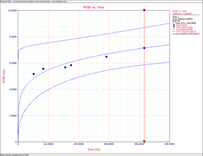
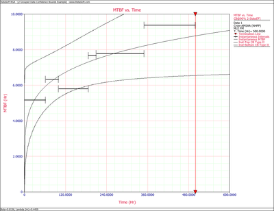
- 2) The Fisher Matrix confidence bounds for the cumulative MTBF and the instantaneous MTBF at the 90% 2-sided confidence level and for [math]\displaystyle{ T=500 }[/math] hr are:
- [math]\displaystyle{ \begin{align} & {{[{{m}_{c}}(T)]}_{L}}= & {{{\hat{m}}}_{c}}(t){{e}^{{{z}_{\alpha /2}}\sqrt{Var({{{\hat{m}}}_{c}}(t))}/{{{\hat{m}}}_{c}}(t)}} \\ & = & 5.8680 \\ & {{[{{m}_{c}}(T)]}_{U}}= & {{{\hat{m}}}_{c}}(t){{e}^{-{{z}_{\alpha /2}}\sqrt{Var({{{\hat{m}}}_{c}}(t))}/{{{\hat{m}}}_{c}}(t)}} \\ & = & 8.6947 \end{align} }[/math]
- and:
- [math]\displaystyle{ \begin{align} & {{[MTB{{F}_{i}}]}_{L}}= & {{{\hat{m}}}_{i}}(t){{e}^{{{z}_{\alpha /2}}\sqrt{Var({{{\hat{m}}}_{i}}(t))}/{{{\hat{m}}}_{i}}(t)}} \\ & = & 6.6483 \\ & {{[MTB{{F}_{i}}]}_{U}}= & {{{\hat{m}}}_{i}}(t){{e}^{-{{z}_{\alpha /2}}\sqrt{Var({{{\hat{m}}}_{i}}(t))}/{{{\hat{m}}}_{i}}(t)}} \\ & = & 11.5932 \end{align} }[/math]
Figures 4fig810 and 4fig811 show plots of the Fisher Matrix confidence bounds for the cumulative and instantaneous MTBF.
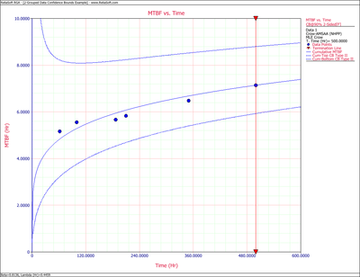
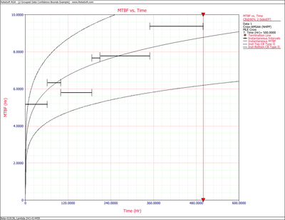
The Crow confidence bounds for the cumulative and instantaneous MTBF at the 90% 2-sided confidence level and for hours are:
- [math]\displaystyle{ T=500 }[/math]
- [math]\displaystyle{ \begin{align} & {{[{{m}_{c}}(T)]}_{L}}= & \frac{1}{C{{(t)}_{U}}} \\ & = & 5.85449 \\ & {{[{{m}_{c}}(T)]}_{U}}= & \frac{1}{C{{(t)}_{L}}} \\ & = & 8.79822 \end{align} }[/math]
- and:
- [math]\displaystyle{ \begin{align} & {{[MTB{{F}_{i}}]}_{L}}= & {{\widehat{m}}_{i}}(1-W) \\ & = & 6.19623 \\ & {{[MTB{{F}_{i}}]}_{U}}= & {{\widehat{m}}_{i}}(1+W) \\ & = & 11.36223 \end{align} }[/math]
Figures 4fig812 and 4fig813 show plots of the Crow confidence bounds for the cumulative and instantaneous MTBF.


