Template:Demonstration test design

Demonstration Test Design

Frequently, a manufacturer will have to demonstrate that a certain product has met a goal of a certain reliability at a given time with a specific confidence. Often, it will be desired to demonstrate that this goal has been met with a zero-failure test. In order to design and conduct such a test, something about the behavior of the product will need to be known, i.e. the shape parameter of the product's life distribution. Beyond this, nothing more about the test is known, and usually the engineer designing the test will have to study the financial trade-offs between the number of units and amount of test time needed to demonstrate the desired goal. In cases like this, it is useful to have a ``carpet plot that shows the possibilities of how a certain specification can be met.

This methodology requires the use of the cumulative binomial distribution in addition to the assumed distribution of the products' lifetimes. Not only does the life distribution of the products need to be assumed beforehand, but a reasonable assumption of the distribution's shape parameter must be provided as well. Additional information that must be supplied includes the reliability to be demonstrated, the confidence level at which the demonstration takes place, the acceptable number of failures and either the number of available units or the amount of available test time. The output of this analysis can be the amount of time required to test the available units or the required number of units that need to be tested during the available test time.

Reliability Demonstration

Frequently, the entire purpose of designing a test with few or no failures is to demonstrate a certain reliability, [math]\displaystyle{ {{R}_{DEMO}} }[/math] , at a certain time. With the exception of the exponential distribution (and ignoring the location parameter for the time being), this reliability is going to be a function of time, a shape parameter and a scale parameter.

[math]\displaystyle{ {{R}_{DEMO}}=g({{t}_{DEMO}};\theta ,\phi ) }[/math]

where:

[math]\displaystyle{ \begin{align} & & {{t}_{DEMO}}\text{ is the time at which the demonstrated reliability is specified} \\ & & \theta \text{ is the shape parameter} \\ & & \phi \text{ is the scale parameter} \end{align} }[/math]

Since required inputs to the process include [math]\displaystyle{ {{R}_{DEMO}} }[/math] , [math]\displaystyle{ {{t}_{DEMO}} }[/math] and [math]\displaystyle{ \theta }[/math] , the value of the scale parameter can be backed out of the reliability equation of the assumed distribution, and will be used in the calculation of another reliability value, [math]\displaystyle{ {{R}_{TEST}} }[/math] , which is the reliability that is going to be incorporated in the actual test calculation. How this calculation is performed depends on whether one is attempting to solve for the number of units to be tested in an available amount of time, or attempting to find how long to test an available number of test units.

Determining Units for Available Test Time

If one knows that the test is to last a certain amount of time, [math]\displaystyle{ {{t}_{TEST}} }[/math] , the number of units that must be tested to demonstrate the specification must be determined. The first step in accomplishing this involves calculating the [math]\displaystyle{ {{R}_{TEST}} }[/math] value.

This should be a simple procedure since:

[math]\displaystyle{ {{R}_{TEST}}=g({{t}_{TEST}};\theta ,\phi ) }[/math]

and [math]\displaystyle{ {{t}_{DEMO}} }[/math] , [math]\displaystyle{ \theta }[/math] and [math]\displaystyle{ \phi }[/math] are already known, and it is just a matter of plugging these values into the appropriate reliability equation.

We now incorporate a form of the cumulative binomial distribution in order to solve for the required number of units. This form of the cumulative binomial appears as:

[math]\displaystyle{ 1-CL=\underset{i=0}{\overset{f}{\mathop \sum }}\,\frac{n!}{i!\cdot (n-i)!}\cdot {{(1-{{R}_{TEST}})}^{i}}\cdot R_{TEST}^{(n-i)} }[/math]

where:

[math]\displaystyle{ \begin{align} & CL= & \text{the required confidence level} \\ & f= & \text{the allowable number of failures} \\ & n= & \text{the total number of units on test} \\ & {{R}_{TEST}}= & \text{the reliability on test} \end{align} }[/math]

Since [math]\displaystyle{ CL }[/math] and [math]\displaystyle{ f }[/math] are required inputs to the process and [math]\displaystyle{ {{R}_{TEST}} }[/math] has already been calculated, it merely remains to solve the cumulative binomial equation for [math]\displaystyle{ n }[/math] , the number of units that need to be tested.

Determining Test Time for Available Units

The way that one determines the test time for the available number of test units is quite similar to the process described previously. In this case, one knows beforehand the number of units, [math]\displaystyle{ n }[/math] , the number of allowable failures, [math]\displaystyle{ f }[/math] , and the confidence level, [math]\displaystyle{ CL }[/math] . With this information, the next step involves solving Eqn. (relcum) for [math]\displaystyle{ {{R}_{TEST}} }[/math] . With this value known, one can use the appropriate reliability equation to back out the value of [math]\displaystyle{ {{t}_{TEST}} }[/math] , since [math]\displaystyle{ {{R}_{TEST}}=g({{t}_{TEST}};\theta ,\phi ) }[/math] , and [math]\displaystyle{ {{R}_{TEST}} }[/math] , [math]\displaystyle{ \theta }[/math] and [math]\displaystyle{ \phi }[/math] have already been calculated or specified.

MTTF Demonstration

Designing a test to demonstrate a certain value of the [math]\displaystyle{ MTTF }[/math] is identical to designing a reliability demonstration test, with the exception of how the value of the scale parameter [math]\displaystyle{ \phi }[/math] is determined. Given the value of the [math]\displaystyle{ MTTF }[/math] and the value of the shape parameter [math]\displaystyle{ \theta }[/math] , the value of the scale parameter [math]\displaystyle{ \phi }[/math] can be calculated. With this, the analysis can proceed as with the reliability demonstration methodology.

Weibull Distribution Example - Demonstrate Reliability

In this example, we will design a test to demonstrate a reliability of 90% at [math]\displaystyle{ t=100 }[/math] hours, with a 95% confidence. We will assume a Weibull distribution with a shape parameter [math]\displaystyle{ \beta =1.5 }[/math] . No failures will be allowed on this test, or [math]\displaystyle{ f=0 }[/math] .

Determining Units for Available Time

In the above scenario, we know that we have the testing facilities available for [math]\displaystyle{ t=48 }[/math] hours. We must now determine the number of units to test for this amount of time with no failures in order to have demonstrated our reliability goal. The first step is to determine the Weibull scale parameter, [math]\displaystyle{ \eta . }[/math] The Weibull reliability equation is:

[math]\displaystyle{ R={{e}^{-{{(t/\eta )}^{\beta }}}} }[/math]

This can be rewritten as:

[math]\displaystyle{ \eta =\frac{{{t}_{DEMO}}}{{{(-\text{ln}({{R}_{DEMO}}))}^{\tfrac{1}{\beta }}}} }[/math]

Since we know the values of [math]\displaystyle{ {{t}_{DEMO}} }[/math] , [math]\displaystyle{ {{R}_{DEMO}} }[/math] and [math]\displaystyle{ \beta }[/math] , we can substitute these in the equation and solve for [math]\displaystyle{ \eta }[/math] :

[math]\displaystyle{ \eta =\frac{100}{{{(-\text{ln}(0.9))}^{\tfrac{1}{1.5}}}}=448.3 }[/math]

Next, the value of [math]\displaystyle{ {{R}_{TEST}} }[/math] is calculated by:

[math]\displaystyle{ {{R}_{TEST}}={{e}^{-{{({{t}_{TEST}}/\eta )}^{\beta }}}}={{e}^{-{{(48/448.3)}^{1.5}}}}=0.966=96.6%. }[/math]

The last step is to substitute the appropriate values into the cumulative binomial equation, which for the Weibull distribution appears as:

[math]\displaystyle{ 1-C.L.=\underset{i=0}{\overset{f}{\mathop \sum }}\,\frac{n!}{i!\cdot (n-i)!}\cdot {{(1-{{e}^{-{{({{t}_{TEST}}/\eta )}^{\beta }}}})}^{i}}\cdot {{({{e}^{-{{({{t}_{TEST}}/\eta )}^{\beta }}}})}^{(n-i)}} }[/math]

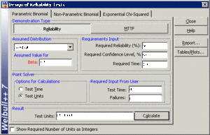
The values of [math]\displaystyle{ CL }[/math] , [math]\displaystyle{ {{t}_{TEST}} }[/math] , [math]\displaystyle{ \beta }[/math] , [math]\displaystyle{ f }[/math] and [math]\displaystyle{ \eta }[/math] have already been calculated or specified, so it merely remains to solve the equation for [math]\displaystyle{ n. }[/math] This value is [math]\displaystyle{ n=85.4994, }[/math] or [math]\displaystyle{ n=86 }[/math] units, since the fractional value must be rounded up to the next integer value. This example solved in Weibull++ is shown next.

Determining Time for Available Units

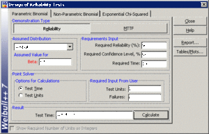
In this case, we will assume that we have 20 units to test, [math]\displaystyle{ n=20 }[/math] , and must determine the test time, [math]\displaystyle{ {{t}_{TEST}}. }[/math] We have already determined the value of the scale parameter, [math]\displaystyle{ \eta }[/math] , in the previous example. Since we know the values of [math]\displaystyle{ n }[/math] , [math]\displaystyle{ CL }[/math] , [math]\displaystyle{ f }[/math] , [math]\displaystyle{ \eta }[/math] and [math]\displaystyle{ \beta }[/math] , it remains to solve Eqn. (weibcum) for [math]\displaystyle{ {{t}_{TEST}} }[/math] . This value is [math]\displaystyle{ {{t}_{TEST}}=126.4339 }[/math] hours. This example solved in Weibull++ is shown next.

Weibull Distribution Example - Demonstrate MTTF

In this example, we will design a test to demonstrate [math]\displaystyle{ MTTF=75 }[/math] hours, with a 95% confidence. We will once again assume a Weibull distribution with a shape parameter [math]\displaystyle{ \beta =1.5 }[/math] . No failures will be allowed on this test, or [math]\displaystyle{ f=0 }[/math] . We want to determine the number of units to test for [math]\displaystyle{ {{t}_{TEST}}=60 }[/math] hours to demonstrate this goal.

The first step in this case involves determining the value of the scale parameter [math]\displaystyle{ \eta }[/math] from the [math]\displaystyle{ MTTF }[/math] equation. The equation for the [math]\displaystyle{ MTTF }[/math] for the Weibull distribution is:

[math]\displaystyle{ MTTF=\eta \cdot \Gamma (1+\frac{1}{\beta }) }[/math]

where [math]\displaystyle{ \Gamma (x) }[/math] is the gamma function of [math]\displaystyle{ x }[/math] . This can be rearranged in terms of .. :

[math]\displaystyle{ \eta =\frac{MTTF}{\Gamma (1+\tfrac{1}{\beta })} }[/math]

Since [math]\displaystyle{ MTTF }[/math] and [math]\displaystyle{ \beta }[/math] have been specified, it is a relatively simple matter to calculate [math]\displaystyle{ \eta =83.1 }[/math] . From this point on, the procedure is the same as the reliability demonstration example. Next, the value of [math]\displaystyle{ {{R}_{TEST}} }[/math] is calculated as:

[math]\displaystyle{ {{R}_{TEST}}={{e}^{-{{({{t}_{TEST}}/\eta )}^{\beta }}}}={{e}^{-{{(60/83.1)}^{1.5}}}}=0.541=54.1% }[/math]

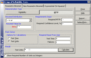
The last step is to substitute the appropriate values into the cumulative binomial equation. The values of [math]\displaystyle{ CL }[/math] , [math]\displaystyle{ {{t}_{TEST}} }[/math] , [math]\displaystyle{ \beta }[/math] , [math]\displaystyle{ f }[/math] and [math]\displaystyle{ \eta }[/math] have already been calculated or specified, so it merely remains to solve Eqn. (relcum) for [math]\displaystyle{ n. }[/math] The value is calculated as [math]\displaystyle{ n=4.8811, }[/math] or [math]\displaystyle{ n=5 }[/math] units, since the fractional value must be rounded up to the next integer value. This example solved in Weibull++ is shown next.

The procedure for determining the required test time proceeds in the same manner, determining [math]\displaystyle{ \eta }[/math] from the [math]\displaystyle{ MTTF }[/math] equation, and following the previously described methodology to determine [math]\displaystyle{ {{t}_{TEST}} }[/math] from Eqn. (weibcum).

Nonparametric Test Design

Eqn. (relcum) can be used for nonparametric demonstration test design. One must merely assume values for three of the inputs of [math]\displaystyle{ CL }[/math] , [math]\displaystyle{ {{R}_{TEST}} }[/math] , [math]\displaystyle{ n }[/math] , and [math]\displaystyle{ f }[/math] , and solve for the fourth. Note that there is no time value associated with this methodology, so one must assume that the value of [math]\displaystyle{ {{R}_{TEST}} }[/math] is associated with the amount of time for which the units were tested.