Template:Lognormal distribution Likelihood ratio confidence bounds
Likelihood Ratio Confidence Bounds
Bounds on Parameters
As covered in Chapter 5, the likelihood confidence bounds are calculated by finding values for [math]\displaystyle{ {{\theta }_{1}} }[/math] and [math]\displaystyle{ {{\theta }_{2}} }[/math] that satisfy:
- [math]\displaystyle{ -2\cdot \text{ln}\left( \frac{L({{\theta }_{1}},{{\theta }_{2}})}{L({{\widehat{\theta }}_{1}},{{\widehat{\theta }}_{2}})} \right)=\chi _{\alpha ;1}^{2} }[/math]
This equation can be rewritten as:
- [math]\displaystyle{ L({{\theta }_{1}},{{\theta }_{2}})=L({{\widehat{\theta }}_{1}},{{\widehat{\theta }}_{2}})\cdot {{e}^{\tfrac{-\chi _{\alpha ;1}^{2}}{2}}} }[/math]
For complete data, the likelihood formula for the normal distribution is given by:
- [math]\displaystyle{ L({\mu }',{{\sigma }_{{{T}'}}})=\underset{i=1}{\overset{N}{\mathop \prod }}\,f({{x}_{i}};{\mu }',{{\sigma }_{{{T}'}}})=\underset{i=1}{\overset{N}{\mathop \prod }}\,\frac{1}{{{x}_{i}}\cdot {{\sigma }_{{{T}'}}}\cdot \sqrt{2\pi }}\cdot {{e}^{-\tfrac{1}{2}{{\left( \tfrac{\text{ln}({{x}_{i}})-{\mu }'}{{{\sigma }_{{{T}'}}}} \right)}^{2}}}} }[/math]
where the [math]\displaystyle{ {{x}_{i}} }[/math] values represent the original time-to-failure data. For a given value of [math]\displaystyle{ \alpha }[/math] , values for [math]\displaystyle{ {\mu }' }[/math] and [math]\displaystyle{ {{\sigma }_{{{T}'}}} }[/math] can be found which represent the maximum and minimum values that satisfy Eqn. (lratio3). These represent the confidence bounds for the parameters at a confidence level [math]\displaystyle{ \delta , }[/math] where [math]\displaystyle{ \alpha =\delta }[/math] for two-sided bounds and [math]\displaystyle{ \alpha =2\delta -1 }[/math] for one-sided.
Example 5
Five units are put on a reliability test and experience failures at 45, 60, 75, 90, and 115 hours. Assuming a lognormal distribution, the MLE parameter estimates are calculated to be [math]\displaystyle{ {{\widehat{\mu }}^{\prime }}=4.2926 }[/math] and [math]\displaystyle{ {{\widehat{\sigma }}_{{{T}'}}}=0.32361. }[/math] Calculate the two-sided 75% confidence bounds on these parameters using the likelihood ratio method.
Solution to Example 5
The first step is to calculate the likelihood function for the parameter estimates:
where [math]\displaystyle{ {{x}_{i}} }[/math] are the original time-to-failure data points. We can now rearrange Eqn. (lratio3) to the form:
- [math]\displaystyle{ L({\mu }',{{\sigma }_{{{T}'}}})-L({{\widehat{\mu }}^{\prime }},{{\widehat{\sigma }}_{{{T}'}}})\cdot {{e}^{\tfrac{-\chi _{\alpha ;1}^{2}}{2}}}=0 }[/math]
Since our specified confidence level, [math]\displaystyle{ \delta }[/math] , is 75%, we can calculate the value of the chi-squared statistic, [math]\displaystyle{ \chi _{0.75;1}^{2}=1.323303. }[/math] We can now substitute this information into the equation:
- [math]\displaystyle{ \begin{align} & L({\mu }',{{\sigma }_{{{T}'}}})-L({{\widehat{\mu }}^{\prime }},{{\widehat{\sigma }}_{{{T}'}}})\cdot {{e}^{\tfrac{-\chi _{\alpha ;1}^{2}}{2}}}= & 0 \\ & L({\mu }',{{\sigma }_{{{T}'}}})-1.115256\times {{10}^{-10}}\cdot {{e}^{\tfrac{-1.323303}{2}}}= & 0 \\ & L({\mu }',{{\sigma }_{{{T}'}}})-5.754703\times {{10}^{-11}}= & 0 \end{align} }[/math]
It now remains to find the values of [math]\displaystyle{ {\mu }' }[/math] and [math]\displaystyle{ {{\sigma }_{{{T}'}}} }[/math] which satisfy this equation. This is an iterative process that requires setting the value of [math]\displaystyle{ {{\sigma }_{{{T}'}}} }[/math] and finding the appropriate values of [math]\displaystyle{ {\mu }' }[/math] , and vice versa.
The following table gives the values of [math]\displaystyle{ {\mu }' }[/math] based on given values of [math]\displaystyle{ {{\sigma }_{{{T}'}}} }[/math] .
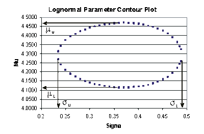
These points are represented graphically in the following contour plot:
(Note that this plot is generated with degrees of freedom [math]\displaystyle{ k=1 }[/math] , as we are only determining bounds on one parameter. The contour plots generated in Weibull++ are done with degrees of freedom [math]\displaystyle{ k=2 }[/math] , for use in comparing both parameters simultaneously.) As can be determined from the table the lowest calculated value for [math]\displaystyle{ {\mu }' }[/math] is 4.1145, while the highest is 4.4708. These represent the two-sided 75% confidence limits on this parameter. Since solutions for the equation do not exist for values of [math]\displaystyle{ {{\sigma }_{{{T}'}}} }[/math] below 0.24 or above 0.48, these can be considered the two-sided 75% confidence limits for this parameter. In order to obtain more accurate values for the confidence limits on [math]\displaystyle{ {{\sigma }_{{{T}'}}} }[/math] , we can perform the same procedure as before, but finding the two values of [math]\displaystyle{ \sigma }[/math] that correspond with a given value of [math]\displaystyle{ {\mu }'. }[/math] Using this method, we find that the 75% confidence limits on [math]\displaystyle{ {{\sigma }_{{{T}'}}} }[/math] are 0.23405 and 0.48936, which are close to the initial estimates of 0.24 and 0.48.
Bounds on Time and Reliability
In order to calculate the bounds on a time estimate for a given reliability, or on a reliability estimate for a given time, the likelihood function needs to be rewritten in terms of one parameter and time/reliability, so that the maximum and minimum values of the time can be observed as the parameter is varied. This can be accomplished by substituting a form of the normal reliability equation into the likelihood function. The normal reliability equation can be written as:
- [math]\displaystyle{ R=1-\Phi \left( \frac{\text{ln}(t)-{\mu }'}{{{\sigma }_{{{T}'}}}} \right) }[/math]
This can be rearranged to the form:
- [math]\displaystyle{ {\mu }'=\text{ln}(t)-{{\sigma }_{{{T}'}}}\cdot {{\Phi }^{-1}}(1-R) }[/math]
where [math]\displaystyle{ {{\Phi }^{-1}} }[/math] is the inverse standard normal. This equation can now be substituted into Eqn. (lognormlikelihood) to produce a likelihood equation in terms of [math]\displaystyle{ {{\sigma }_{{{T}'}}}, }[/math] [math]\displaystyle{ t }[/math] and [math]\displaystyle{ R\ \ : }[/math]
- [math]\displaystyle{ L({{\sigma }_{{{T}'}}},t/R)=\underset{i=1}{\overset{N}{\mathop \prod }}\,\frac{1}{{{x}_{i}}\cdot {{\sigma }_{{{T}'}}}\cdot \sqrt{2\pi }}\cdot {{e}^{-\tfrac{1}{2}{{\left( \tfrac{\text{ln}({{x}_{i}})-\left( \text{ln}(t)-{{\sigma }_{{{T}'}}}\cdot {{\Phi }^{-1}}(1-R) \right)}{{{\sigma }_{{{T}'}}}} \right)}^{2}}}} }[/math]
The unknown variable [math]\displaystyle{ t/R }[/math] depends on what type of bounds are being determined. If one is trying to determine the bounds on time for a given reliability, then [math]\displaystyle{ R }[/math] is a known constant and [math]\displaystyle{ t }[/math] is the unknown variable. Conversely, if one is trying to determine the bounds on reliability for a given time, then [math]\displaystyle{ t }[/math] is a known constant and [math]\displaystyle{ R }[/math] is the unknown variable. Either way, Eqn. (lognormliketr) can be used to solve Eqn. (lratio3) for the values of interest.
Example 6
For the data given in Example 5, determine the two-sided 75% confidence bounds on the time estimate for a reliability of 80%. The ML estimate for the time at [math]\displaystyle{ R(t)=80% }[/math] is 55.718.
Solution to Example 6
In this example, we are trying to determine the two-sided 75% confidence bounds on the time estimate of 55.718. This is accomplished by substituting [math]\displaystyle{ R=0.80 }[/math] and [math]\displaystyle{ \alpha =0.75 }[/math] into Eqn. (lognormliketr), and varying [math]\displaystyle{ {{\sigma }_{{{T}'}}} }[/math] until the maximum and minimum values of [math]\displaystyle{ t }[/math] are found. The following table gives the values of [math]\displaystyle{ t }[/math] based on given values of [math]\displaystyle{ {{\sigma }_{{{T}'}}} }[/math] .
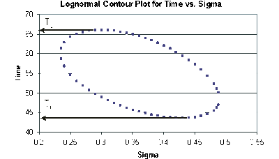
This data set is represented graphically in the following contour plot:
As can be determined from the table, the lowest calculated value for [math]\displaystyle{ t }[/math] is 43.634, while the highest is 66.085. These represent the two-sided 75% confidence limits on the time at which reliability is equal to 80%.
Example 7
For the data given in Example 5, determine the two-sided 75% confidence bounds on the reliability estimate for [math]\displaystyle{ t=65 }[/math] . The ML estimate for the reliability at [math]\displaystyle{ t=65 }[/math] is 64.261%.
Solution to Example 7
In this example, we are trying to determine the two-sided 75% confidence bounds on the reliability estimate of 64.261%. This is accomplished by substituting [math]\displaystyle{ t=65 }[/math] and [math]\displaystyle{ \alpha =0.75 }[/math] into Eqn. (lognormliketr), and varying [math]\displaystyle{ {{\sigma }_{{{T}'}}} }[/math] until the maximum and minimum values of [math]\displaystyle{ R }[/math] are found. The following table gives the values of [math]\displaystyle{ R }[/math] based on given values of [math]\displaystyle{ {{\sigma }_{{{T}'}}} }[/math] .
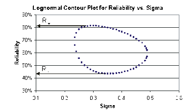
This data set is represented graphically in the following contour plot:
As can be determined from the table, the lowest calculated value for [math]\displaystyle{ R }[/math] is 43.444%, while the highest is 81.508%. These represent the two-sided 75% confidence limits on the reliability at [math]\displaystyle{ t=65 }[/math] .


