Fleet Analysis Example
New format available! This reference is now available in a new format that offers faster page load, improved display for calculations and images and more targeted search.
As of January 2024, this Reliawiki page will not continue to be updated. Please update all links and bookmarks to the latest references at RGA examples and RGA reference examples.
This example appears in the Reliability Growth and Repairable System Analysis Reference.
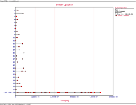
The following table presents data for a fleet of 27 systems. A cycle is a complete history from overhaul to overhaul. The failure history for the last completed cycle for each system is recorded. This is a random sample of data from the fleet. These systems are in the order in which they were selected. Suppose the intervals to group the current data are 10,000; 20,000; 30,000; 40,000 and the final interval is defined by the termination time. Conduct the fleet analysis.
| Sample Fleet Data | |||
| System | Cycle Time [math]\displaystyle{ {{T}_{j}}\,\! }[/math] | Number of failures [math]\displaystyle{ {{N}_{j}}\,\! }[/math] | Failure Time [math]\displaystyle{ {{X}_{ij}}\,\! }[/math] |
|---|---|---|---|
| 1 | 1396 | 1 | 1396 |
| 2 | 4497 | 1 | 4497 |
| 3 | 525 | 1 | 525 |
| 4 | 1232 | 1 | 1232 |
| 5 | 227 | 1 | 227 |
| 6 | 135 | 1 | 135 |
| 7 | 19 | 1 | 19 |
| 8 | 812 | 1 | 812 |
| 9 | 2024 | 1 | 2024 |
| 10 | 943 | 2 | 316, 943 |
| 11 | 60 | 1 | 60 |
| 12 | 4234 | 2 | 4233, 4234 |
| 13 | 2527 | 2 | 1877, 2527 |
| 14 | 2105 | 2 | 2074, 2105 |
| 15 | 5079 | 1 | 5079 |
| 16 | 577 | 2 | 546, 577 |
| 17 | 4085 | 2 | 453, 4085 |
| 18 | 1023 | 1 | 1023 |
| 19 | 161 | 1 | 161 |
| 20 | 4767 | 2 | 36, 4767 |
| 21 | 6228 | 3 | 3795, 4375, 6228 |
| 22 | 68 | 1 | 68 |
| 23 | 1830 | 1 | 1830 |
| 24 | 1241 | 1 | 1241 |
| 25 | 2573 | 2 | 871, 2573 |
| 26 | 3556 | 1 | 3556 |
| 27 | 186 | 1 | 186 |
| Total | 52110 | 37 | |
Solution
The sample fleet data set can be grouped into 10,000; 20,000; 30,000; 40,000 and 52,110 time intervals. The following table gives the grouped data.
| Grouped Data | |
| Time | Observed Failures |
|---|---|
| 10,000 | 8 |
| 20,000 | 16 |
| 30,000 | 22 |
| 40,000 | 27 |
| 52,110 | 37 |
Based on the above time intervals, the maximum likelihood estimates of [math]\displaystyle{ \widehat{\lambda }\,\! }[/math] and [math]\displaystyle{ \widehat{\beta }\,\! }[/math] for this data set are then given by:
- [math]\displaystyle{ \begin{matrix} \widehat{\lambda }=0.00147 \\ \widehat{\beta }=0.93328 \\ \end{matrix}\,\! }[/math]
The next figure shows the System Operation plot.

